Last updated: September 6, 2018
The Emissions Modeling Framework (EMF) is a software system designed to solve many long-standing difficulties of emissions modeling identified at EPA. The overall process of emissions modeling involves gathering measured or estimated emissions data into emissions inventories; applying growth and controls information to create future year and controlled emissions inventories; and converting emissions inventories into hourly, gridded, chemically speciated emissions estimates suitable for input into air quality models such as the Community Multiscale Air Quality (CMAQ) model.
This User’s Guide focuses on the data management and analysis capabilities of the EMF. The EMF also contains a Control Strategy Tool (CoST) for developing future year and controlled emissions inventories and is capable of driving SMOKE to develop CMAQ inputs.
Many types of data are involved in the emissions modeling process including:
Quality assurance (QA) is an important component of emissions modeling. Emissions inventories and other modeling data must be analyzed and reviewed for any discrepancies or outlying data points. Data files need to be organized and tracked so changes can be monitored and updates made when new data is available. Running emissions modeling software such as the Sparse Matrix Operator Kernel Emissions (SMOKE) Modeling System requires many configuration options and input files that need to be maintained so that modeling output can be reproduced in the future. At all stages, coordinating tasks and sharing data between different groups of people can be difficult and specialized knowledge may be required to use various tools.
In your emissions modeling work, you may have found yourself asking questions like:
The EMF helps with these issues by using a client-server system where emissions modeling information is centrally stored and can be accessed by multiple users. The EMF integrates quality control processes into its data management to help with development of high quality emissions results. The EMF also organizes emissions modeling data and tracks emissions modeling efforts to aid in reproducibility of emissions modeling results. Additionally, the EMF strives to allow non-experts to use emissions modeling capabilities such as future year projections, spatial allocation, chemical speciation, and temporal allocation.
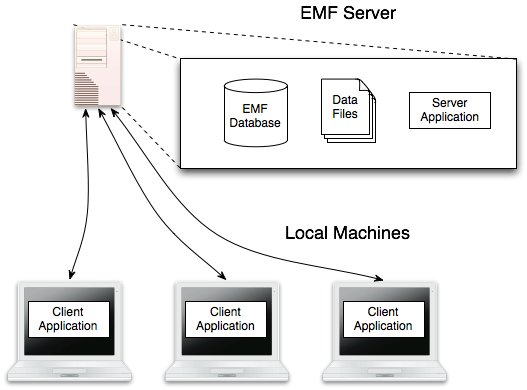
A typical installation of the EMF system is illustrated in Fig. 1.1. In this case, a group of users shares a single EMF server with multiple local machines running the client application. The EMF server consists of a database, file storage, and the server application which handles requests from the clients and communicates with the database. The client application runs on each user’s computer and provides a graphical interface for interacting with the emissions modeling data stored on the server (see Sec. 2). Each user has his or her own username and password for accessing the EMF server. Some users will have administrative privileges which allow them to access additional system data such as managing users or dataset types.
For a simpler setup, all of the EMF components can be run on a single machine: database, server application, and client application. With this “all-in-one” setup, the emissions data would generally not be shared between multiple users.
Fig. 1.2 illustrates the basic workflow of data in the EMF system.
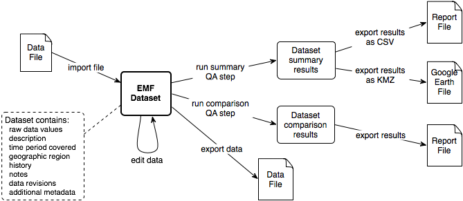
Emissions modeling data files are imported into the EMF system where they are represented as datasets (see Sec. 3). The EMF supports many different types of data files including emissions inventories, allocation factors, cross-reference files, and reference data. Each dataset matches a dataset type which defines the format of the data to be loaded from the file (Sec. 3.2). In addition to the raw data values, the EMF stores various metadata about each dataset including the time period covered, geographic region, the history of the data, and data usage in model runs or QA analysis.
Once your data is stored as a dataset, you can review and edit the dataset’s properties (Sec. 3.5) or the data itself (Sec. 3.6) using the EMF client. You can also run QA steps on a dataset or set of datasets to extract summary information, compare datasets, or convert the data to a different format (see Sec. 4).
You can export your dataset to a file and download it to your local computer (Sec. 3.8). You can also export reports that you create with QA steps for further analysis in a spreadsheet program or to create charts (Sec. 4.5).
The EMF client is a graphical desktop application written in Java. While it is primarily developed and used in Windows, it will run under Mac OS X and Linux (although due to font differences the window layout may not be optimal). The EMF client can be run on Windows 7, Windows 8, or Windows 10.
The EMF requires Java 7 or greater. The following instructions will help you check if you have Java installed on your Windows machine and what version is installed. If you need more details, please visit How to find Java version in Windows [java.com].
The latest version(s) of Java on your system will be listed as Java 7 with an associated Update number (eg. Java 7 Update 21). Older versions may be listed as Java(TM), Java Runtime Environment, Java SE, J2SE or Java 2.
Windows 8
Windows 7 and Vista
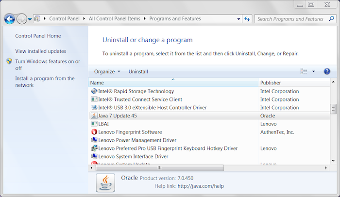
Fig. 2.1 shows the Programs and Features Control Panel on Windows 7 with Java installed. The installed version of Java is Version 7 Update 45; this version does not need to be updated to run the EMF client.
If you need to install Java, please follow the instructions for downloading and installing Java for a Windows computer [java.com]. Note that you will need administrator privileges to install Java on Windows. During the installation, make a note of the directory where Java is installed on your computer. You will need this information to configure the EMF client.
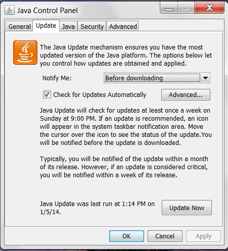
If Java is installed on your computer but is not version 7 or greater, you will need to update your Java installation. Start by opening the Java Control Panel from the Windows Control Panel. Fig. 2.2 shows the Java Control Panel.
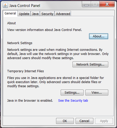
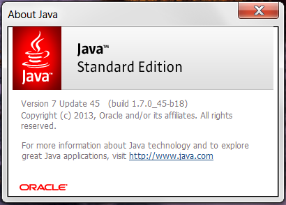
Clicking the About button will display the Java version dialog seen in Fig. 2.3. In Fig. 2.3, the installed version of Java is Version 7 Update 45. This version of Java does not need to be updated to run the EMF client.
To update Java, click the tab labeled Update in the Java Control Panel (see Fig. 2.4). Click the button labeled Update Now in the bottom right corner of the Java Control Panel to update your installation of Java.
How you install the EMF client depends on which EMF server you will be connecting to. To download and install an all-in-one package that includes all the EMF components, please visit https://www.cmascenter.org/cost/. Other users should contact their EMF server administrators for instructions on downloading and installing the EMF client.
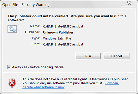
To launch the EMF client, double-click the file named EMFClient.bat. You may see a security warning similar to Fig. 2.5. Uncheck the box labeled “Always ask before opening this file” to avoid the warning in the future.
When you start the EMF client application, you will initially see a login window like Fig. 2.6.
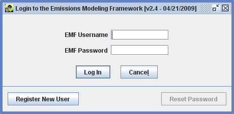
If you are an existing EMF user, enter your EMF username and password in the login window and click the Log In button. If you forget your password, an EMF Administrator can reset it for you. Note: The Reset Password button is used to update your password when it expires; it can’t be used if you’ve lost your password. See Sec. 2.5 for more information on password expiration.
If you have never used the EMF before, click the Register New User button to bring up the Register New User window as shown in Fig. 2.7.
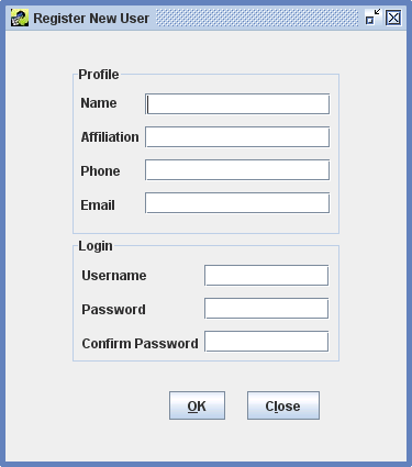
In the Register New User window, enter the following information:
Click OK to create your account. If there are any problems with the information you entered, an error message will be displayed at the top of the window as shown in Fig. 2.8.
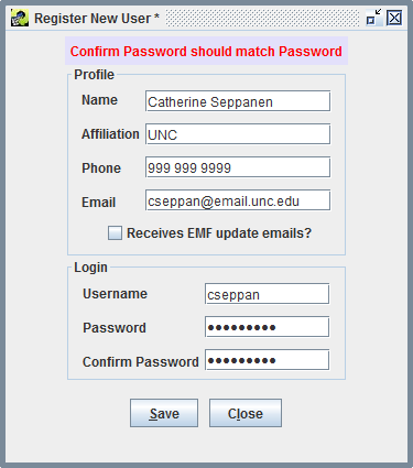
Once you have corrected any errors, your account will be created and the EMF main window will be displayed (Fig. 2.9).
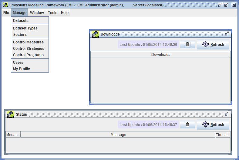
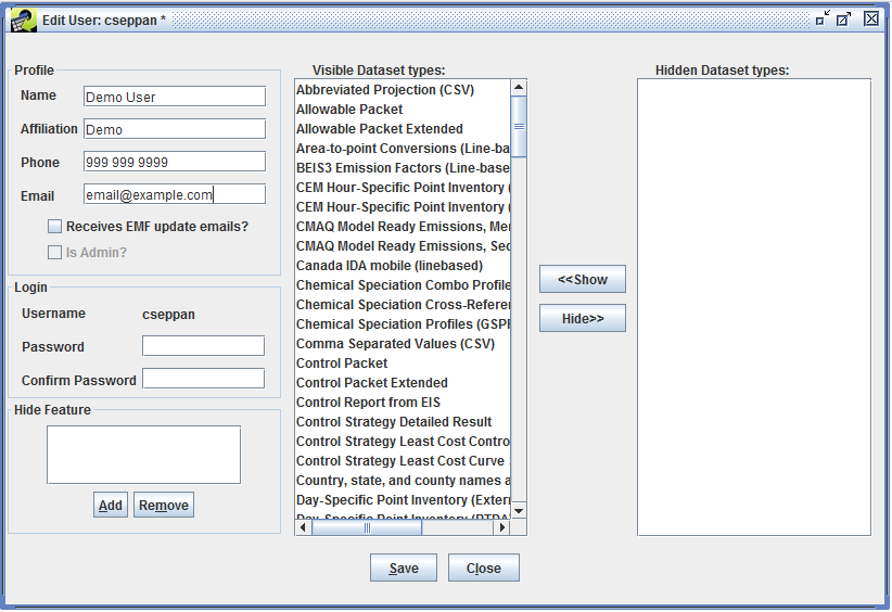
If you need to update any of your profile information or change your password, click the Manage menu and select My Profile to bring up the Edit User window shown in Fig. 2.10.
To change your password, enter your new password in the Password field and be sure to enter the same password in the Confirm Password field. Your password must be at least 8 characters long and must contain at least one digit.
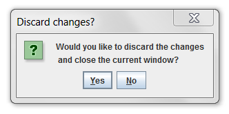
Once you have entered any updated information, click the Save button to save your changes and close the Edit User window. You can close the window without saving changes by clicking the Close button. If you have unsaved changes, you will be asked to confirm that you want to discard your changes (Fig. 2.11).
Passwords in the EMF expire every 90 days. If you try to log in and your password has expired, you will see the message “Password has expired. Reset Password.” as shown in Fig. 2.12.
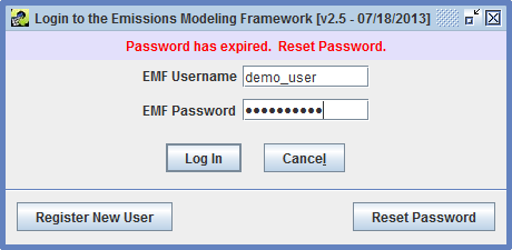
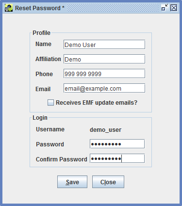
Click the Reset Password button to set a new password as shown in Fig. 2.13. After entering your new password and confirming it, click the Save button to save your new password and you will be logged in to the EMF. Make sure to use your new password next time you log in.
As you become familiar with the EMF client application, you’ll encounter various concepts that are reused through the interface. In this section, we’ll briefly introduce these concepts. You’ll see specific examples in the following chapters of this guide.
First, we’ll discuss the difference between viewing an item and editing an item. Viewing something in the EMF means that you are just looking at it and can’t change its information. Conversely, editing an item means that you have the ability to change something. Oftentimes, the interface for viewing vs. editing will look similar but when you’re just viewing an item, various fields won’t be editable. For example, Fig. 2.14 shows the Dataset Properties View window while Fig. 2.15 shows the Dataset Properties Editor window for the same dataset.
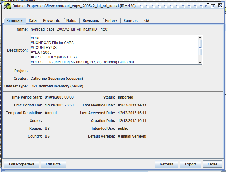
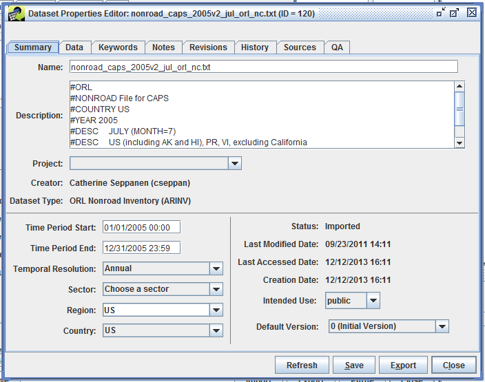
In the edit window, you can make various changes to the dataset like editing the dataset name, selecting the temporal resolution, or changing the geographic region. Clicking the Save button will save your changes. In the viewing window, those same fields are not editable and there is no Save button. Notice in the lower left hand corner of Fig. 2.14 the button labeled Edit Properties. Clicking this button will bring up the editing window shown in Fig. 2.15.
Similarly, Fig. 2.16 shows the QA tab of the Dataset Properties View as compared to Fig. 2.17 showing the same QA tab but in the Dataset Properties Editor.
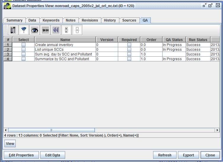
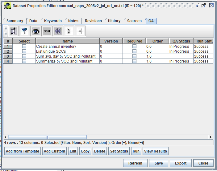
In the View window, the only option is to view each QA step whereas the Editor allows you to interact with the QA steps by adding, editing, copying, deleting, or running the steps. If you are having trouble finding an option you’re looking for, check to see if you’re viewing an item vs. editing it.
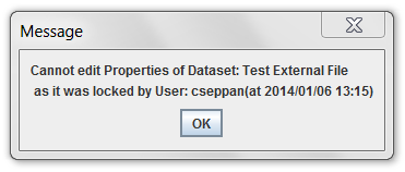
Only one user can edit a given item at a time. Thus, if you are editing a dataset, you have a “lock” on it and no one else will be able to edit it at the same time. Other users will be able to view the dataset as you’re editing it. If you try to edit a locked dataset, the EMF will display a message like Fig. 2.18. For some items in the EMF, you may only be able to edit the item if you created it or if your account has administrative privileges.
Generally you will need to click the Save button to save changes that you make. If you have unsaved changes and click the Close button, you will be asked if you want to discard your changes as shown in Fig. 2.11. This helps to prevent losing your work if you accidentally close a window.
The EMF client application loads data from the EMF server. As you and other users work, your information is saved to the server. In order to see the latest information from other users, the client application needs to refresh its information by contacting the server. The latest data will be loaded from the server when you open a new window. If you are working in an already open window, you may need to click on the Refresh button to load the newest data. Fig. 2.19 highlights the Refresh button in the Dataset Manager window. Clicking Refresh will contact the server and load the latest list of datasets.
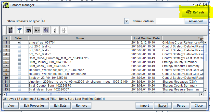
Various windows in the EMF client application have Refresh buttons, usually in either the top right corner as in Fig. 2.19 or in the row of buttons on the bottom right like in Fig. 2.17.
You will also need to use the Refresh button if you have made changes and return to a previously opened window. For example, suppose you select a dataset in the Dataset Manager and edit the dataset’s name as described in Sec. 3.5. When you save your changes, the previously opened Dataset Manager window won’t automatically display the updated name. If you close and re-open the Dataset Manager, the dataset’s name will be refreshed; otherwise, you can click the Refresh button to update the display.
Many actions in the EMF are run on the server. For example, when you run a QA step, the client application on your computer sends a message to the server to start running the step. Depending on the type of QA step, this processing can take a while and so the client will allow you to do other work while it periodically checks with the server to find out the status of your request. These status checks are displayed in the Status Window shown in Fig. 2.20.
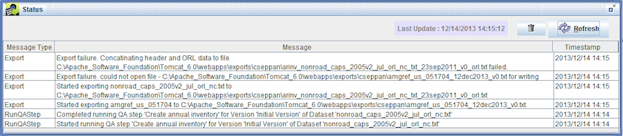
The status window will show you messages about tasks when they are started and completed. Also, error messages will be displayed if a task could not be completed. You can click the Refresh button in the Status Window to refresh the status. The Trash icon clears the Status Window.
Most lists of data within the EMF are displayed using the Sort-Filter-Select Table, a generic table that allows sorting, filtering, and selection (as the name suggests). Fig. 2.21 shows the sort-filter-select table used in the Dataset Manager. (To follow along with the figures, select the main Manage menu and then select Datasets. In the window that appears, find the Show Datasets of Type pull-down menu near the top of the window and select All.)
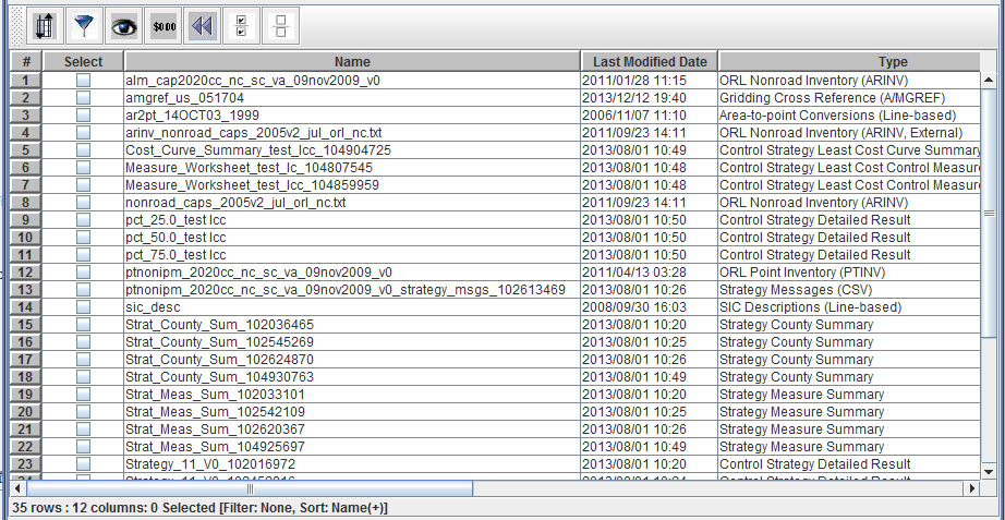
Row numbers are shown in the first column, while the first row displays column headers. The column labeled Select allows you to select individual rows by checking the box in the column. Selections are used for different activities depending on where the table is displayed. For example, in the Dataset Manager window you can select various datasets and then click the View button to view the dataset properties of each selected dataset. In other contexts, you may have options to change the status of all the selected items or copy the selected items. There are toolbar buttons to allow you to quickly select all items in a table (Sec. 2.6.12) and to clear all selections (Sec. 2.6.13).
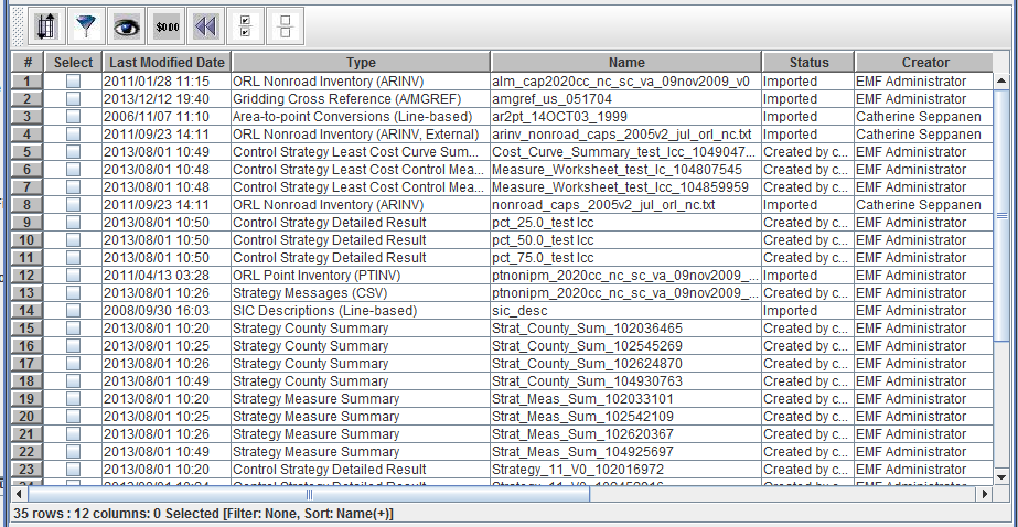
The horizontal scroll bar at the bottom indicates that there are more columns in the table than fit in the window. Scroll to the right in order to see all the columns as in Fig. 2.22.
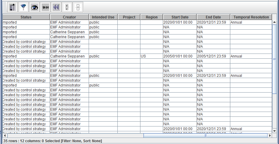
Notice the info line displayed at the bottom of the table. In Fig. 2.22 the line reads 35 rows : 12 columns: 0 Selected [Filter: None, Sort: None]. This line gives information about the total number of rows and columns in the table, the number of selected items, and any filtering or sorting applied.
Columns can be resized by clicking on the border between two column headers and dragging it right or left. Your mouse cursor will change to a horizontal double-headed arrow when resizing columns.
You can rearrange the order of the columns in the table by clicking a column header and dragging the column to a new position. Fig. 2.23 shows the sort-filter-select table with columns rearranged and resized.
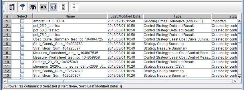
To sort the table using data from a given column, click on the column header such as Last Modified Date. Fig. 2.24 shows the table sorted by Last Modified Date in descending order (latest dates first). The table info line now includes Sort: Last Modified Date(-).
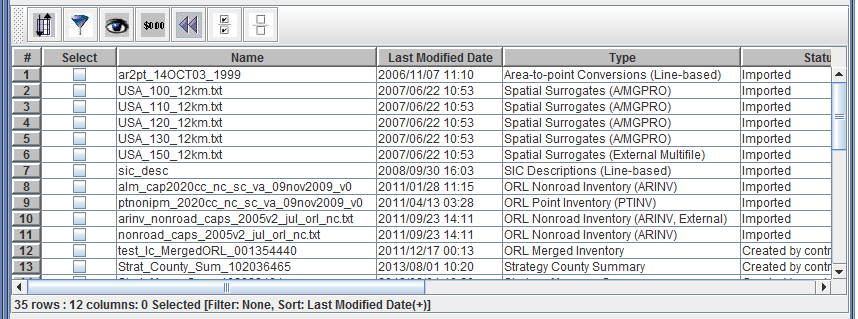
If you click the Last Modified Date header again, the table will re-sort by Last Modified Date in ascending order (earliest dates first). The table info line also changes to Sort: Last Modified Date(+) as seen in Fig. 2.25.
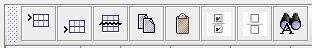
The toolbar at the top of the table (as shown in Fig. 2.26) has buttons for the following actions (from left to right):

If you hover your mouse over any of the buttons, a tooltip will pop up to remind you of each button’s function.

The Sort toolbar button brings up the Sort Columns dialog as shown in Fig. 2.27. This dialog allows you to sort the table by multiple columns and also allows case sensitive sorting. (Quick sorting by clicking a column header uses case insensitive sorting.)
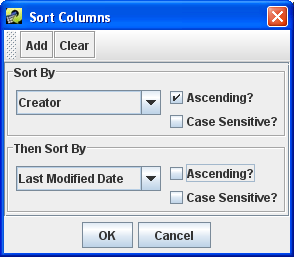
In the Sort Columns Dialog, select the first column you would use to sort the data from the Sort By pull-down menu. You can also specify if the sort order should be ascending or descending and if the sort comparison should be case sensitive.
To add additional columns to sort by, click the Add button and then select the column in the new Then Sort By pull-down menu. When you have finished setting up your sort selections, click the OK button to close the dialog and re-sort the table. The info line beneath the table will show all the columns used for sorting like Sort: Creator(+), Last Modified Date(-).
To remove your custom sorting, click the Clear button in the Sort Columns dialog and then click the OK button. You can also use the Reset toolbar button to reset all custom settings as described in Sec. 2.6.11.

The Filter Rows toolbar button brings up the Filter Rows dialog as shown in Fig. 2.28. This dialog allows you to create filters to “whittle down” the rows of data shown in the table. You can filter the table’s rows based on any column with several different value matching options.
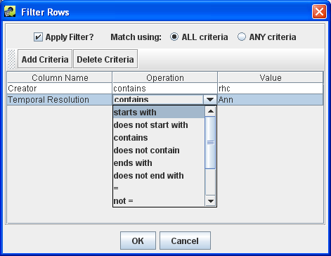
To add a filter criterion, click the Add Criteria button and a new row will appear in the dialog window. Clicking the cell directly under the Column Name header displays a pull-down menu to pick which column you would like use to filter the rows. The Operation column allows you to select how the filter should be applied; for example, you can filter for data that starts with the given value or does not contain the value. Finally, click the cell under the Value header and type in the value to use. Note that the filter values are case-sensitive. A filter value of “nonroad” would not match the dataset type “ORL Nonroad Inventory”.
If you want to specify additional criteria, click Add Criteria again and follow the same process. To remove a filter criterion, click on the row you want to remove and then click the Delete Criteria button.
If the radio button labeled Match using: is set to ALL criteria, then only rows that match all the specified criteria will be shown in the filtered table. If Match using: is set to ANY criteria, then rows will be shown if they meet any of the criteria listed.
Once you are done specifying your filter options, click the OK button to close the dialog and return to the filtered table. The info line beneath the table will include your filter criteria like Filter: Creator contains rhc, Temporal Resolution starts with Ann.
To remove your custom filtering, you can delete the filter criteria from the Filter Rows dialog or uncheck the Apply Filter? checkbox to turn off the filtering without deleting your filter rules. You can also use the Reset toolbar button to reset all custom settings as described in Sec. 2.6.11. Note that clicking the Reset button will delete your filter rules.

The Show/Hide Columns toolbar button brings up the Show/Hide Columns dialog as shown in Fig. 2.29. This dialog allows you to customize which columns are displayed in the table.
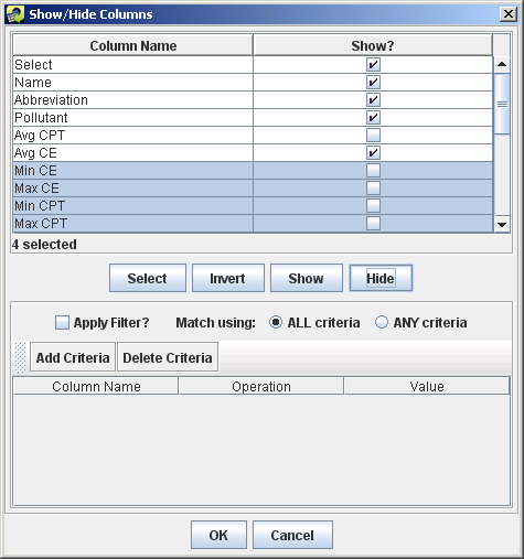
To hide a column, uncheck the box next to the column name under the Show? column. Click the OK button to return to the table. The columns you unchecked will no longer be seen in the table. The info line beneath the table will also be updated with the current number of displayed columns.
To make a hidden column appear again, open the Show/Hide Columns dialog and check the Show? box next to the hidden column’s name. Click OK to close the Show/Hide Columns dialog.
To select multiple columns to show or hide, click on the first column name of interest. Then hold down the Shift key and click a second column name to select it and the intervening columns. Once rows are selected, clicking the Show or Hide buttons in the middle of the dialog will check or uncheck all the Show? boxes for the selected rows. To select multiple rows that aren’t next to each other, you can hold down the Control key while clicking each row. The Invert button will invert the selected rows. After checking/unchecking the Show? checkboxes, click OK to return to the table with the columns shown/hidden as desired.
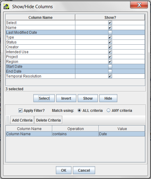
The Show/Hide Columns dialog also supports filtering to find columns to show or hide. This is an infrequently used option most useful for locating columns to show or hide when there are many columns in the table. Fig. 2.30 shows an example where a filter has been set up to match column names that contain the value “Date”. Clicking the Select button above the filtering options selects matching rows which can then be hidden by clicking the Hide button.

The Format Columns toolbar button displays the Format Columns dialog show in Fig. 2.31. This dialog allows you to customize the formatting of columns. In practice, this dialog is not used very often but it can be helpful to format numeric data by changing the number of decimal places or the number of significant digits shown.
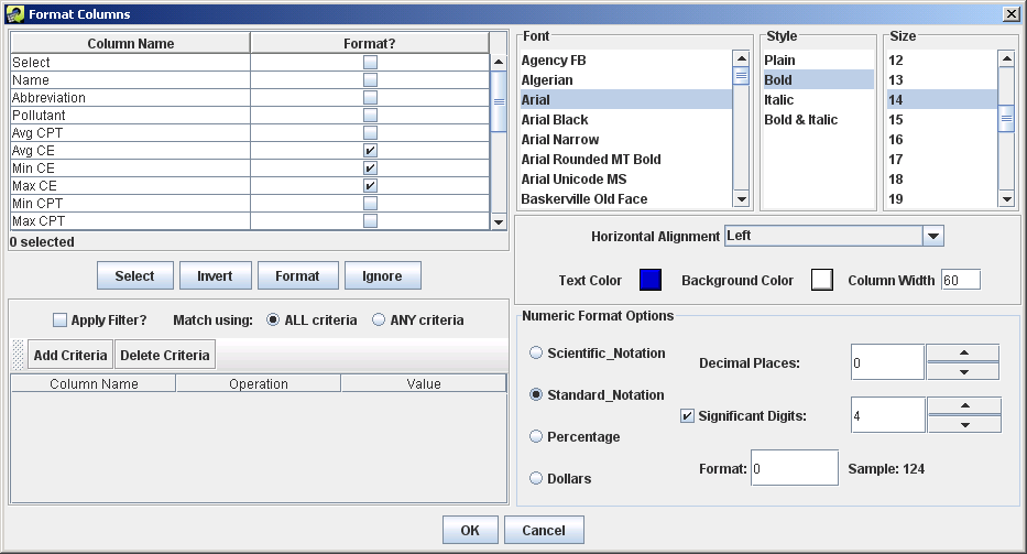
To change the format of a column, first check the checkbox next to the column name in the Format? column. If you only select columns that contain numeric data, the Numeric Format Options section of the dialog will appear; otherwise, it will not be visible. The Format Columns dialog supports filtering by column name similar to the Show/Hide Columns dialog (Sec. 2.6.9).
From the Format Columns dialog, you can change the font, the style of the font (e.g. bold, italic), the horizontal alignment for the column (e.g. left, center, right), the text color, and the column width. For numeric columns, you can specify the number of significant digits and decimal places.

The Reset toolbar button will remove all customizations from the table: sorting, filtering, hidden columns, and formatting. It will also reset the column order and set column widths back to the default.

The Select All toolbar button selects all the rows in the table. After clicking the Select All button, you will see that the checkboxes in the Select column are now all checked. You can select or deselect an individual item by clicking its checkbox in the Select column.
![]()
The Clear All Selections toolbar button unselects all the rows in the table.
Emissions inventories, reference data, and other types of data files are imported into the EMF and stored as datasets. A dataset encompasses both the data itself as well as various dataset properties such as the time period covered by the dataset and geographic extent of the dataset. Changes to a dataset are tracked as dataset revisions. Multiple versions of the data for a dataset can be stored in the EMF.
Each dataset has a dataset type. The dataset type describes the format of the dataset’s data. For example, the dataset type for an ORL Point Inventory (PTINV) defines the various data fields of the inventory file such as FIPS code, SCC code, pollutant name, and annual emissions value. A different dataset type like Spatial Surrogates (A/MGPRO) defines the fields in the corresponding file: surrogate code, FIPS code, grid cell, and surrogate fraction.
The EMF also supports flexible dataset types without fixed format - Comma Separated Value and Line-based. These types allow for new kinds of data to be loaded into the EMF without requiring updates to the EMF software.
When importing data into the EMF, you can choose between internal dataset types where the data itself is stored in the EMF database and external dataset types where the data remains in a file on disk and the EMF only tracks the metadata. For internal datasets, the EMF provides data editing, revision and version tracking, and data analysis using SQL queries. External datasets can be used to track files that don’t need these features or data that can’t be loaded into the EMF like binary NetCDF files.
You can view the dataset types defined in the EMF by selecting Dataset Types from the main Manage menu. EMF administrators can add, edit, and remove dataset types; non-administrative users can view the dataset types. Fig. 3.1 shows the Dataset Type Manager.
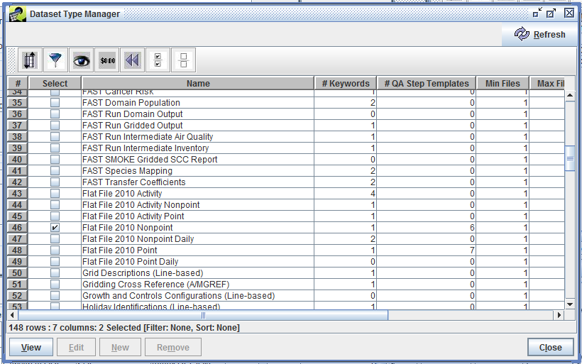
To view the details of a particular dataset type, check the box next to the type you want to view (for example, “Flat File 2010 Nonpoint”) and then click the View button in the bottom left-hand corner.
Fig. 3.2 shows the View Dataset Type window for the Flat File 2010 Nonpoint dataset type. Each dataset type has a name and a description along with metadata about who created the dataset type and when, and also the last modified date for the dataset type.
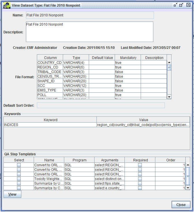
The dataset type defines the format of the data file as seen in the File Format section of Fig. 3.2. For the Flat File 2010 Nonpoint dataset type, the columns from the raw data file are mapped into columns in the database when the data is imported. Each data column must match the type (string, integer, floating point) and can be mandatory or optional.
Keyword-value pairs can be used to give the EMF more information about a dataset type. Tbl. 3.1 lists some of the keywords available. Sec. 3.5.3 provides more information about using and adding keywords.
| Keyword | Description | Example |
|---|---|---|
| EXPORT_COLUMN_LABEL | Indicates if columns labels should be included when exporting the data to a file | FALSE |
| EXPORT_HEADER_COMMENTS | Indicates if header comments should be included when exporting the data to a file | FALSE |
| EXPORT_INLINE_COMMENTS | Indicates if inline comments should be included when exporting the data to a file | FALSE |
| EXPORT_PREFIX | Filename prefix to include when exporting the data to a file | ptinv_ |
| EXPORT_SUFFIX | Filename suffix to use when exporting the data to a file | .csv |
| INDICES | Tells the system to create indices in the database on the given columns | region_cd|country_cd|scc |
| REQUIRED_HEADER | Indicates a line that must occur in the header of a data file | #FORMAT=FF10_ACTIVITY |
Each dataset type can have QA step templates assigned. These are QA steps that apply to any dataset of the given type. More information about using QA step templates in given in Sec. 4.
Dataset types can be added, edited, or deleted by EMF administrators. In this section, we list dataset types that are commonly used. Your EMF installation may not include all of these types or may have additional types defined.
| Dataset Type Name | Description | Link to File Format |
|---|---|---|
| Flat File 2010 Activity | Onroad mobile activity data (VMT, VPOP, speed) in Flat File 2010 (FF10) format | SMOKE documentation |
| Flat File 2010 Activity Nonpoint | Nonpoint activity data in FF10 format | Same format as Flat File 2010 Activity |
| Flat File 2010 Activity Point | Point activity data in FF10 format | Not available |
| Flat File 2010 Nonpoint | Nonpoint or nonroad emissions inventory in FF10 format | SMOKE documentation |
| Flat File 2010 Nonpoint Daily | Nonpoint or nonroad day-specific emissions inventory in FF10 format | SMOKE documentation |
| Flat File 2010 Point | Point emissions inventory in FF10 format | SMOKE documentation |
| Flat File 2010 Point Daily | Point day-specific emissions inventory in FF10 format | SMOKE documentation |
| ORL Day-Specific Fires Data Inventory (PTDAY) | Day-specific fires inventory | SMOKE documentation |
| ORL Fire Inventory (PTINV) | Wildfire and prescribed fire inventory | SMOKE documentation |
| ORL Nonpoint Inventory (ARINV) | Nonpoint emissions inventory in ORL format | SMOKE documentation |
| ORL Nonroad Inventory (ARINV) | Nonroad emissions inventory in ORL format | SMOKE documentation |
| ORL Onroad Inventory (MBINV) | Onroad mobile emissions inventory in ORL format | SMOKE documentation |
| ORL Point Inventory (PTINV) | Point emissions inventory in ORL format | SMOKE documentation |
| Dataset Type Name | Description | Link to File Format |
|---|---|---|
| Country, state, and county names and data (COSTCY) | List of region names and codes with default time zones and daylight-saving time flags | SMOKE documentation |
| Grid Descriptions (Line-based) | List of projections and grids | I/O API documentation |
| Holiday Identifications (Line-based) | Holidays date list | SMOKE documentation |
| Inventory Table Data (INVTABLE) | Pollutant reference data | SMOKE documentation |
| MACT description (MACTDESC) | List of MACT codes and descriptions | SMOKE documentation |
| NAICS description file (NAICSDESC) | List of NAICS codes and descriptions | SMOKE documentation |
| ORIS Description (ORISDESC) | List of ORIS codes and descriptions | SMOKE documentation |
| Point-Source Stack Replacements (PSTK) | Replacement stack parameters | SMOKE documentation |
| SCC Descriptions (Line-based) | List of SCC codes and descriptions | SMOKE documentation |
| SIC Descriptions (Line-based) | List of SIC codes and descriptions | SMOKE documentation |
| Surrogate Descriptions (SRGDESC) | List of surrogate codes and descriptions | SMOKE documentation |
| Dataset Type Name | Description | Link to File Format |
|---|---|---|
| Area-to-point Conversions (Line-based) | Point locations to assign to stationary area and nonroad mobile sources | SMOKE documentation |
| Chemical Speciation Combo Profiles (GSPRO_COMBO) | Multiple speciation profile combination data | SMOKE documentation |
| Chemical Speciation Cross-Reference (GSREF) | Cross-reference data to match inventory sources to speciation profiles | SMOKE documentation |
| Chemical Speciation Profiles (GSPRO) | Factors to allocate inventory pollutant emissions to model species | SMOKE documentation |
| Gridding Cross Reference (A/MGREF) | Cross-reference data to match inventory sources to spatial surrogates | SMOKE documentation |
| Pollutant to Pollutant Conversion (GSCNV) | Conversion factors when inventory pollutant doesn’t match speciation profile pollutant | SMOKE documentation |
| Spatial Surrogates (A/MGPRO) | Factors to allocate emissions to grid cells | SMOKE documentation |
| Spatial Surrogates (External Multifile) | External dataset type to point to multiple surrogates files on disk | Individual files have same format as Spatial Surrogates (A/MGPRO) |
| Temporal Cross Reference (A/M/PTREF) | Cross-reference data to match inventory sources to temporal profiles | SMOKE documentation |
| Temporal Profile (A/M/PTPRO) | Factors to allocate inventory emissions to hourly estimates | SMOKE documentation |
| Dataset Type Name | Description | Link to File Format |
|---|---|---|
| Allowable Packet | Allowable emissions cap or replacement values | SMOKE documentation |
| Allowable Packet Extended | Allowable emissions cap or replacement values; supports monthly values | Download CSV |
| Control Packet | Control efficiency, rule effectiveness, and rule penetration rate values | SMOKE documentation |
| Control Packet Extended | Control percent reduction values; supports monthly values | Download CSV |
| Control Strategy Detailed Result Extended | Output from CoST | Download CSV |
| Control Strategy Least Cost Control Measure Worksheet | Output from CoST | Not available |
| Control Strategy Least Cost Curve Summary | Output from CoST | Not available |
| Facility Closure Extended | Facility closure dates | Download CSV |
| Projection Packet | Factors to grow emissions values into the past or future | SMOKE documentation |
| Projection Packet Extended | Projection factors; supports monthly values | Download CSV |
| Strategy County Summary | Output from CoST | Not available |
| Strategy Impact Summary | Output from CoST | Not available |
| Strategy Measure Summary | Output from CoST | Not available |
| Strategy Messages (CSV) | Output from CoST | Not available |
The main interface for finding and interacting with datasets is the Dataset Manager. To open the Dataset Manager, select the Manage menu at the top of the EMF main window, and then select the Datasets menu item. It may take a little while for the window to appear. As shown in Fig. 3.3, the Dataset Manager initially does not show any datasets. This is to avoid loading a potentially large list of datasets from the server.
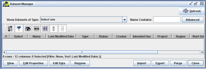
From the Dataset Manager you can:
To quickly find datasets of interest, you can use the Show Datasets of Type pull-down menu at the top of the Dataset Manager window. Select “ORL Point Inventory (PTINV)” and the datasets matching that Dataset Type are loaded into the Dataset Manager as shown in Fig. 3.4.
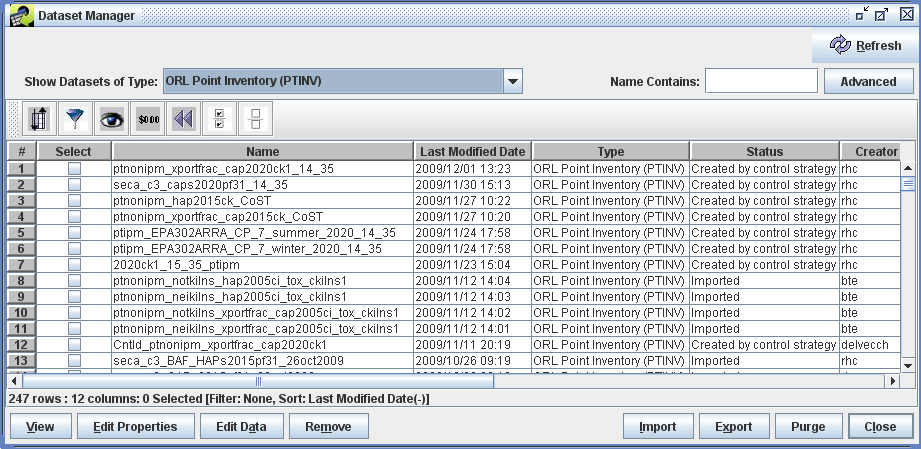
The matching datasets are shown in a table that lists some of their properties, including the dataset’s name, last modified date, dataset type, status indicating how the dataset was created, and the username of the dataset’s creator. Tbl. 3.6 describes each column in the Dataset Manager window. In the Dataset Manager window, use the horizontal scroll bar to scroll the table to the right to see all the columns.
| Column | Description |
|---|---|
| Name | A unique name or label for the dataset. You choose this name when importing data and it can be edited by users with appropriate privileges. |
| Last Modified Date | The most recent date and time when the data (not the metadata) of the dataset was modified. When the dataset is initially imported, the Last Modified Date is set to the file’s timestamp. |
| Type | The Dataset Type of this dataset. The Dataset Type incorporates information about the structure of the data and information regarding how the data can be sorted and summarized. |
| Status | Shows whether the dataset was imported from disk or created in some other way such as an output from a control strategy. |
| Creator | The username of the person who originally created the dataset. |
| Intended Use | Specifies whether the dataset is intended to be public (accessible to any user), private (accessible only to the creator), or to be used by a specific group of users. |
| Project | The name of a study or set of work for which this dataset was created. The project field can help you organize related files. |
| Region | The name of a geographic region to which the dataset applies. |
| Start Date | The start date and time for the data contained in the dataset. |
| End Date | The end date and time for the data contained in the dataset. |
| Temporal Resolution | The temporal resolution of the data contained in the dataset (e.g. annual, daily, or hourly). |
Using the Dataset Manager, you can select datasets of interest by checking the checkboxes in the Select column and then perform various actions related to those datasets. Tbl. 3.7 lists the buttons along the bottom of the Dataset Manager window and describes the actions for each button.
| Command | Description |
|---|---|
| View | Displays a read-only Dataset Properties View for each of the selected datasets. You can view a dataset even when someone else is editing that dataset’s properties or data. |
| Edit Properties | Opens a writeable Dataset Properties Editor for each of the selected datasets. Only one user can edit a dataset at any given time. |
| Edit Data | Opens a Dataset Versions Editor for each of the selected datasets. |
| Remove | Marks each of the selected datasets for deletion. Datasets are not actually deleted until you click purge. |
| Import | Opens the Import Datasets window where you can import data files into the EMF as new datasets. |
| Export | Opens the Export window to write the data for one version of the selected dataset to a file. |
| Purge | Permanently removes any datasets that are marked for deletion from the EMF. |
| Close | Closes the Dataset Manager window. |
There are several ways to find datasets using the Dataset Manager. First, you can show all datasets with a particular dataset type by choosing the dataset type from the Show Datasets of Type menu. If there are more than a couple hundred datasets matching the type you select, the system will warn you and suggest you enter something in the Name Contains field to limit the list.
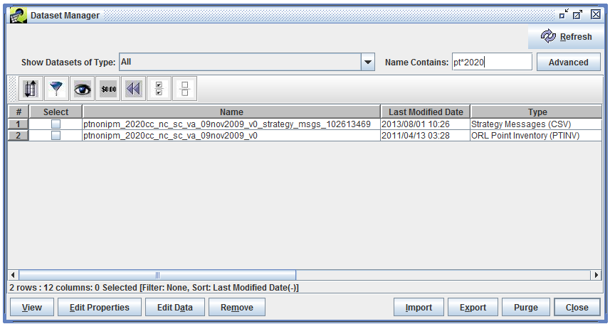
The Name Contains field allows you to enter a search term to match dataset names. For example, if you type 2020 in the textbox and then hit Enter, the Dataset Manager will show all the datasets with “2020” in their names. You can also use wildcards in your keyword. Using the keyword pt*2020 will show all datasets whose name contains “pt” followed at some point by “2020” as shown in Fig. 3.5. The Name Contains search is not case sensitive.
If you want to search for datasets using attributes other than the dataset’s name or using multiple criteria, click the Advanced button. The Advanced Dataset Search dialog as shown in Fig. 3.6 will be displayed.
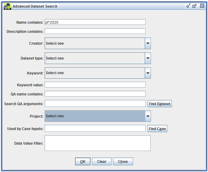
You can use the Advanced Dataset Search to search for datasets based on the contents of the dataset’s description, the dataset’s creator, project, and more. Tbl. 3.8 lists the options for the advanced search.
| Search option | Description |
|---|---|
| Name contains | Performs a case-insensitive search of the dataset name; supports wildcards |
| Description contains | Performs a case-insensitive search of the dataset description; supports wildcards |
| Creator | Matches datasets created by the specified user |
| Dataset type | Matches datasets of the specified type |
| Keyword | Matches datasets that have the specified keyword |
| Keyword value | Matches datasets where the specified keyword has the specified value; must exactly match the dataset’s keyword value (case-insensitive) |
| QA name contains | Performs a case-insensitive search of the names of the QA steps associated with datasets |
| Search QA arguments | Searches the arguments to QA steps associated with datasets |
| Project | Matches datasets assigned to the specified project |
| Used by Case Inputs | Finds datasets by case (not described in this User’s Guide) |
| Data Value Filter | Matches datasets using SQL like “FIPS='37001' and SCC like '102005%'”; must be used with the dataset type criterion |
After setting your search criteria, click OK to perform the search and update the Dataset Manager window. The Advanced Dataset Search dialog will remain visible until you click Close. This allows you to refine your search or perform additional searches if needed. If you specify multiple search criteria, a dataset must satisfy all of the specified criteria to be shown in the Dataset Manager.
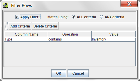
Another option for finding datasets is to use the filtering options of the Dataset Manager. (See Sec. 2.6.8 for a complete description of the Filter Rows dialog.) Filtering helps narrow down the list of datasets already shown in the Dataset Manager. Click the Filter Rows button in the toolbar to bring up the Filter Rows dialog. In the dialog, you can create a filter to show only datasets whose dataset type contains the word “Inventory” (see Fig. 3.7).
Once you’ve entered the filter criteria, click OK to return to the Dataset Manager. The list of datasets has now been reduced to only those matching the filter as shown in Fig. 3.8.
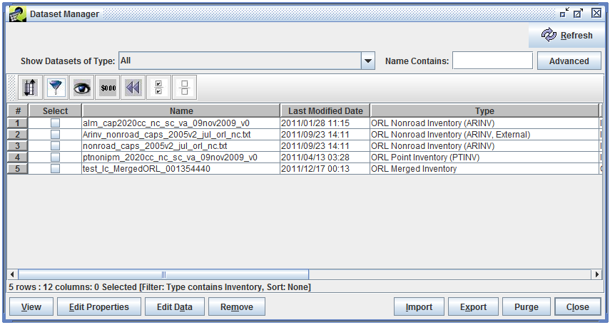
Using filtering allows you to search for datasets using any column shown in the Dataset Manager. Remember that filtering will only apply to the datasets already shown in the table - it doesn’t search the database for additional datasets like the Advanced Dataset Search feature.
To view or edit the properties of a dataset, select the dataset in the Dataset Manager and then click either the View or Edit Properties button at the bottom of the window. The Dataset Properties View or Editor window will be displayed with the Summary tab selected as shown in Fig. 3.9. If multiple datasets are selected, separate Dataset Properties windows will be displayed for each selected dataset.
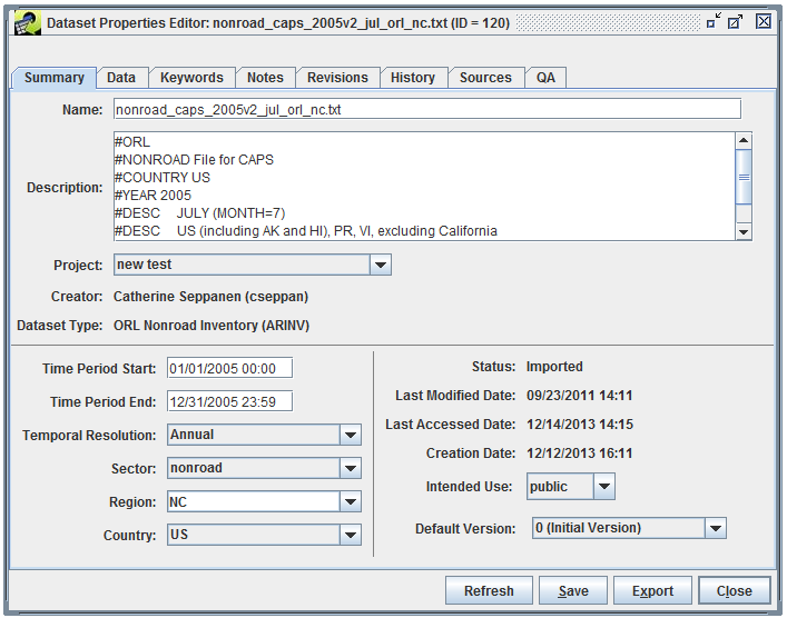
The interface for viewing dataset properties is very similar to the editing interface except that the values are all read-only. In this section, we will show the editing versions of the interface so that all available options are shown. In general, if you don’t need to edit a dataset, it’s better to just view the properties since viewing the dataset doesn’t lock it for editing by another user.
The Dataset Properties window divides its data into several tabs. Tbl. 3.9 gives a brief description of each tab.
| Tab | Description |
|---|---|
| Summary | Shows high-level properties of the dataset |
| Data | Provides access to the actual data stored for the dataset |
| Keywords | Shows additional types of metadata not found on the Summary tab |
| Notes | Shows comments that users have made about the dataset and questions they may have |
| Revisions | Shows the revisions that have been made to the dataset |
| History | Shows how the dataset has been used in the past |
| Sources | Shows where the data came from and where it is stored in the database, if applicable |
| QA | Shows QA steps that have been run using the dataset |
There are several buttons at the bottom of the editor window that appear on all tabs:
The Summary tab of the Dataset Properties Editor (Fig. 3.9) displays high level summary information about the Dataset. Many of these properties are shown in the list of datasets displayed by the Dataset Manager and as a result are described in Tbl. 3.6. The additional properties available in the Summary tab are described in Tbl. 3.10.
| Column | Description |
|---|---|
| Description | Descriptive information about the dataset. The contents of this field are initially populated from the full-line comments found in the header and other sections of the file used to create the dataset when it is imported. Users are free to add on to the contents of this field which is written to the top of the resulting file when the data is exported from the EMF. |
| Sector | The emissions sector to which this data applies. |
| Country | The country to which the data applies. |
| Last Accessed Date | The date/time the data was last exported. |
| Creation Date | The date/time the dataset was created. |
| Default Version | Indicates which version of the dataset is considered to be the default. The default version of a dataset is important in that it indicates to other users and to some quality assurance queries the appropriate version of the dataset to be used. |
Values of text fields (boxes with white background) are changed by typing into the fields. Other properties are set by selecting items from pull-down menus.
Some notes about updating the various editable fields follow:
Name: If you change the dataset name, the EMF will verify that your newly selected name is unique within the EMF.
Description: Be careful updating the description if the file will be exported for use in SMOKE. For example, ORL files must start with #ORL or SMOKE will not accept them. Thus, it is safer to add information to the end of the description.
Project: You may select a different project for the dataset by choosing another item from the pull-down menu. If you are an EMF Administrator, you can create a new project by typing a non-existent value into the editable menu.
Region: You can select an existing region by choosing an item from the pull-down menu or you can type a value into the editable menu to add a new region.
Default Version: Only versions of datasets that have been marked as final can be selected as the default version.
The Data tab of the Dataset Properties Editor (Fig. 3.10) provides access to the actual data stored for the dataset. If the dataset has multiple versions, they will be listed in the Versions table.
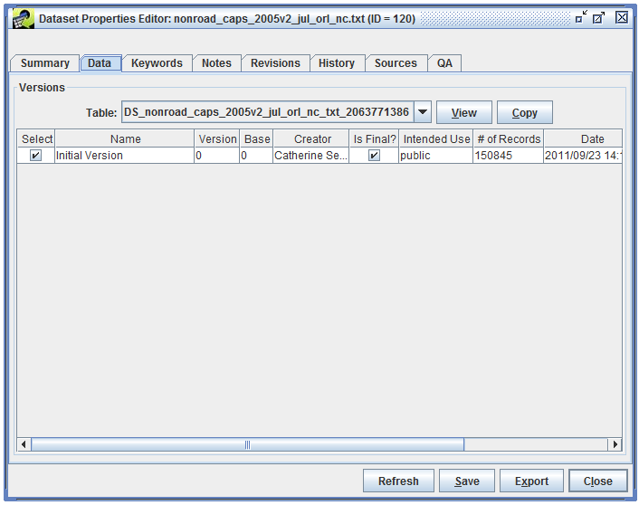
To view the data associated with a particular version, select the version and click the View button. For more information about viewing the raw data, see Sec. 3.6. The Copy button allows you to copy any version of the data marked as final to a new dataset.
The Keywords tab of the Dataset Properties Editor (Fig. 3.11) shows additional types of metadata about the dataset stored as keyword-value pairs.
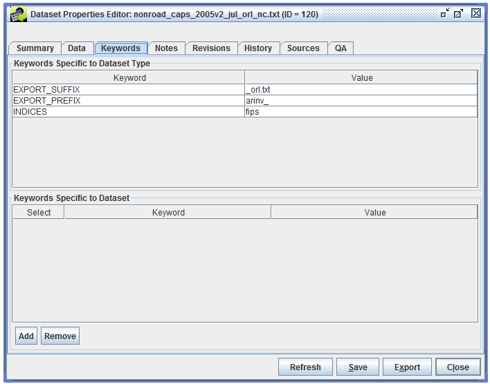
The Keywords Specific to Dataset Type section show keywords associated with the dataset’s type. These keywords are described in Sec. 3.2.
Additional dataset-specific keywords can be added by clicking the Add button. A new entry will be added to the Keyword Specific to Dataset section of the window. Type the keyword and its value in the Keyword and Value cells.
The Notes tab of the Dataset Properties Editor (Fig. 3.12) shows comments that users have made about the dataset and questions they may have. Each note is associated with a particular version of a dataset.
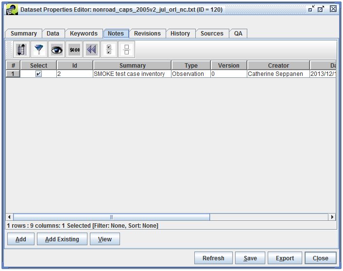
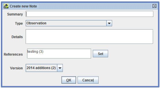
To create a new note about a dataset, click the Add button and the Create New Note dialog will open (Fig. 3.13). Notes can reference other notes so that questions can be answered. Click the Set button to display other notes for this dataset and select any referenced notes.
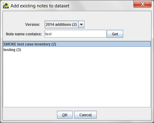
The Add Existing button in the Notes tab opens a dialog to add existing notes to the dataset. This feature is useful if you need to add the same note to a set of files. Add a new note for the first dataset and then for subsequent datasets, use the “Note name contains:” field to search for the newly added note. In the list of matched notes, select the note to add and click the OK button.
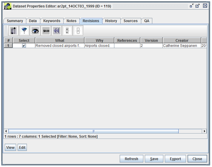
The Revisions tab of the Dataset Properties Editor (Fig. 3.15) shows revisions that have been made to the data contained in the dataset. See Sec. 3.7 for more information about editing the raw data.
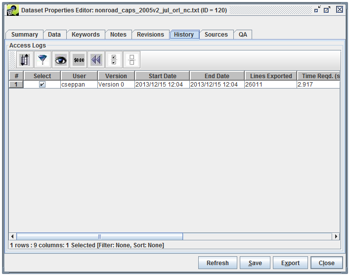
The History tab of the Dataset Properties Editor (Fig. 3.16) shows the export history of the dataset. When the dataset is exported, a history record is automatically created containing the name of the user who exported the data, the version that was exported, the location on the server where the file was exported, and statistics about how many lines were exported and the export time.
The Sources tab of the Dataset Properties Editor (Fig. 3.17) shows where the data associated with the dataset came from and where it is stored in the database, if applicable. For datasets where the data is stored in the EMF database, the Table column shows the name of the table in the EMF database and Source lists the original file the data was imported from.
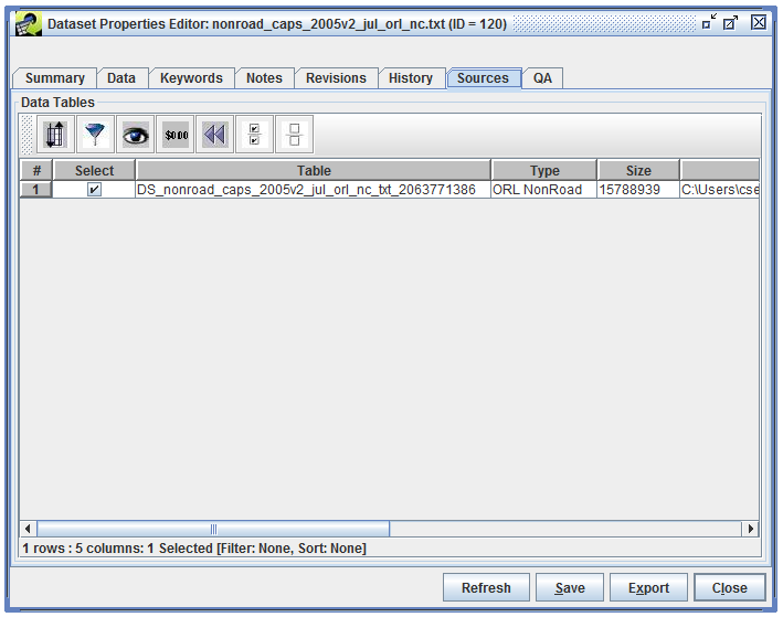
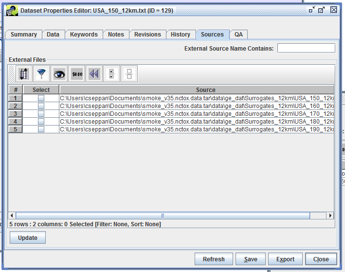
Fig. 3.18 shows the Sources tab for a dataset that references external files. In this case, there is no Table column since the data is not stored in the EMF database. The Source column lists the current location of the external file. If the location of the external file changes, you can click the Update button to browse for the file in its new location.
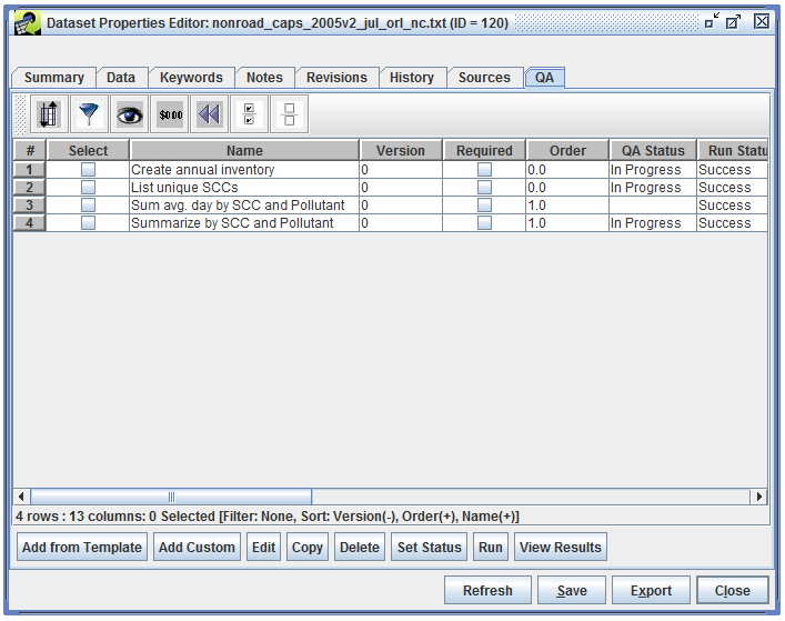
The QA tab of the Dataset Properties Editor (Fig. 3.19) shows the QA steps that have been run using the dataset. See Sec. 4 for more information about setting up and running QA steps.
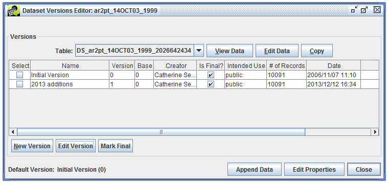
The EMF allows you to view and edit the raw data stored for each dataset. To work with the data, select a dataset from the Dataset Manager and click the Edit Data button to open the Dataset Versions Editor (Fig. 3.20). This window shows the same list of versions as the Dataset Properties Data tab (Sec. 3.5.2).
To view the data, select a version and click the View Data button. The raw data is displayed in the Data Viewer as shown in Fig. 3.21.
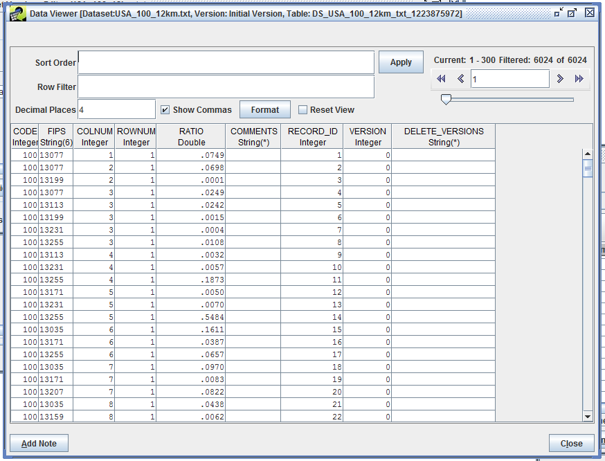
Since the data stored in the EMF may have millions of rows, the client application only transfers a small amount of data (300 rows) from the server to your local machine at a time. The area in the top right corner of the Data Viewer displays information about the currently loaded rows along with controls for paging through the data. The single left and right arrows move through the data one chunk at a time while the double arrows jump to the beginning and end of the data. If you hover your mouse over an arrow, a tooltip will pop up to remind you of its function. The slider allows you to quickly jump to different parts of the data.
You can control how the data are sorted by entering a comma-separated list of columns in the Sort Order field and then clicking the Apply button. A descending sort can be specified by following the column name with desc.
The Row Filter field allows you to enter criteria and filter the rows that are displayed. The syntax is similar to a SQL WHERE clause. Tbl. 3.11 shows some example filters and the syntax for each.
| Filter Purpose | Row Filter Syntax |
|---|---|
| Filter on a particular set of SCCs | scc like '101%' or scc like '102%' |
| Filter on a particular set of pollutants | poll in ('PM10', 'PM2_5') |
| Filter sources only in NC (State FIPS = 37), SC (45), and VA (51); note that FIPS column format is State + County FIPS code (e.g., 37001) |
substring(FIPS,1,2) in ('37', '45', '51') |
| Filter sources only in CA (06) and include only NOx and VOC pollutants | fips like '06%' and (poll = 'NOX' or poll = 'VOC') |
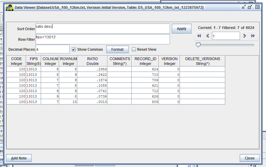
Fig. 3.22 shows the data sorted by the column “ratio” in descending order and filtered to only show rows where the FIPS code is “13013”.
The Row Filter syntax used in the Data Viewer can also be used when exporting datasets to create filtered export files (Sec. 3.8.1. If you would like to create a new dataset based on a filtered existing dataset, you can export your filtered dataset and then import the resulting file as a new dataset. Sec. 3.8 describes exporting datasets and Sec. 3.9 explains how to import datasets.
The EMF does not allow data to be edited after a version has been marked as final. If a dataset doesn’t have a non-final version, first you will need to create a new version. Open the Dataset Versions Editor as shown in Fig. 3.20. Click the New Version button to bring up the Create a New Version dialog window like Fig. 3.23.
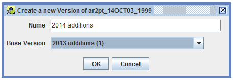
Enter a name for the new version and select the base version. The base version is the starting point for the new version and can only be a version that is marked as final. Click OK to create the new version. The Dataset Versions Editor will show your newly created version (Fig. 3.24).
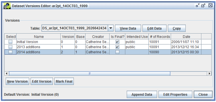
You can now select the non-final version and click the Edit Data button to display the Data Editor as shown in Fig. 3.25.

The Data Editor uses the same paging mechanisms, sort, and filter options as the Data Viewer described in Sec. 3.6. You can double-click a data cell to edit the value. The toolbar shown in Fig. 3.26 provides options for adding and deleting rows.
The functions of each toolbar button are described below, listed left to right:
In the Data Editor window, you can undo your changes by clicking the Discard button. Otherwise, click the Save button to save your changes. If you have made changes, you will need to enter Revision Information before the EMF will allow you to close the window. Revisions for a dataset are shown in the Dataset Properties Revisions tab (see Sec. 3.5.5).
When you export a dataset, the EMF will generate a file containing the data in the format defined by the dataset’s type. To export a dataset, you can either select the dataset in the Dataset Manager window and click the Export button or you can click the Export button in the Dataset Properties window. Either way will open the Export dialog as shown in Fig. 3.28. If you have multiple datasets selected in the Dataset Manager when you click the Export button, the Export dialog will list each dataset in the Datasets field.
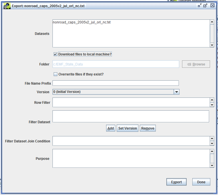
Typically, you will check the Download files to local machine? checkbox. With this option, the EMF will export the dataset to a file on the EMF server and then automatically download it to your local machine. When downloading files to your local machine, the folder input field is not active. The downloaded files will be placed in a temporary directory on your local computer. The EMF property local.temp.dir controls the location of the temporary directory. EMF properties can be edited in the EMFPrefs.txt file. Note that the Overwrite files if they exit? checkbox isn’t functional at this point.
You can enter a prefix to be added to the names of the exported files in the File Name Prefix field. Exported files will be named based on the dataset name and may have prefixes or suffixes attached based on keywords associated with the dataset or dataset type.
If you are exporting a single dataset and that dataset has multiple versions, the Version pull-down menu will allow you to select which version you would like to export. If you are exporting multiple datasets, the default version of each dataset will be exported.
The Row Filter, Filter Dataset, and Filter Dataset Join Condition fields allow for filtering the dataset during export to reduce the total number of rows exported. See Sec. 3.8.1 for more information about these settings.
Before clicking the Export button, enter a Purpose for your export. This will be logged as part of the history for the dataset. If you do not enter any text in the Purpose field, the fact that you exported the dataset will still be logged as part of the dataset’s history. At this time, history records are only created when the Download files to local machine? checkbox is not checked.
After clicking the Export button, check the Status window to see if any problems arise during the export. If the export succeeds, you will see a status message like
Completed export of nonroad_caps_2005v2_jul_orl_nc.txt to <server directory>/nonroad_caps_2005v2_jul_orl_nc.txt in 2.137 seconds. The file will start downloading momentarily, see the Download Manager for the download status.
You can bring up the Downloads window as shown in Fig. 3.29 by opening the Window menu at the top of the EMF main window and selecting Downloads.
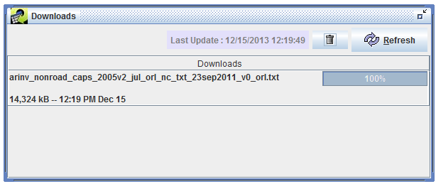
As your file is downloading, the progress bar on the right side of the window will update to show you the progress of the download. Once it reaches 100%, your download is complete. Right click on the filename in the Downloads window and select Open Containing Folder to open the folder where the file was downloaded.
The export filtering options allow you to select and export portions of a dataset based on your matching criteria.
The Row Filter field shown in the Export Dialog in Fig. 3.28 uses the same syntax as the Data Viewer window (Sec. 3.6) and allows you to export only a subset of the data. Example filters are shown in Tbl. 3.11.
Filter Dataset and Filter Dataset Join Condition, also shown in Fig. 3.28, allow for advanced filtering of the dataset using an additional dataset. For example, if you are exporting a nonroad inventory, you can choose to only export rows that match a different inventory by FIPS code or SCC. When you click the Add button, the Select Datasets dialog appears as in Fig. 3.30.
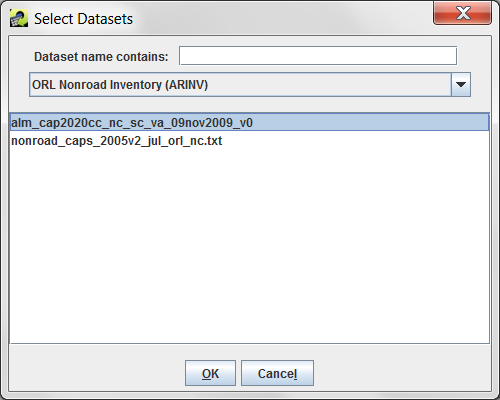
Select the dataset type for the dataset you want to use as a filter from the pull-down menu. You can use the Dataset name contains field to further narrow down the list of matching datasets. Click on the dataset name to select it and then click OK to return to the Export dialog.
The selected dataset is now shown in the Filter Dataset box. If the filter dataset has multiple versions, click the Set Version button to select which version to use for filtering. You can remove the filter dataset by clicking the Remove button.
Next, you will enter the criteria to use for filtering in the Filter Dataset Join Condition textbox. The syntax is similar to a SQL JOIN condition where the left hand side corresponds to the dataset being exported and the right hand side corresponds to the filter dataset. You will need to know the column names you want to use for each dataset.
| Type of Filter | Filter Dataset Join Condition |
|---|---|
| Export records where the FIPS, SCC, and plant IDs are the same in both datasets; both datasets have the same column names |
fips=fips scc=scc plantid=plantid |
| Export records where the SCC, state codes, and pollutants are the same in both datasets; the column names differ between the datasets |
scc=scc_code substring(fips,1,2)=state_cd poll=poll_code |
Once your filter conditions are set up, click the Export button to begin the export. Only records that match all of the filter conditions will be exported. Status messages in the Status window will contain additional information about your filter. If no records match your filter condition, the export will fail and you will see a status message like:
Export failure. ERROR: nonroad_caps_2005v2_jul_orl_nc.txt will not be exported because no records satisfied the filter
If the export succeeds, the status message will include a count of the number of records in the database and the number of records exported:
No. of records in database: 150845; Exported: 26011
Importing a dataset is the process where the EMF reads a data file or set of data files from disk, stores the data in the database (for internal dataset types), and creates metadata about the dataset. To import a dataset, start by clicking the Import button in the bottom right corner of the Dataset Manager window (Fig. 3.4). The Import Datasets dialog will be displayed as shown in Fig. 3.31. You can also bring up the Import Datasets dialog from the main EMF File menu, then select Import.
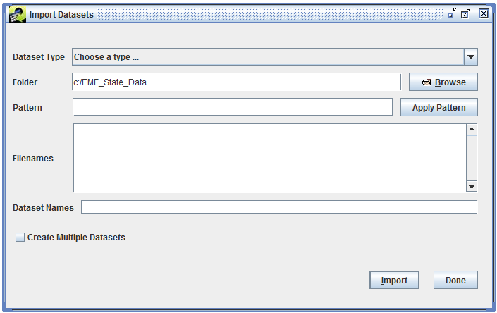
An advantage to opening the Import Datasets dialog from the Dataset Manager as opposed to using the File menu is that if you have a dataset type selected in the Dataset Manager Show Datasets of Type pull-down menu, then that dataset type will automatically be selected for you in the Import Datasets dialog.
In the Import Datasets dialog, first use the Dataset Type pull-down menu to select the dataset type corresponding to the file you want to import. For example, if your data file is a annual point-source emissions inventory in Flat File 2010 (FF10) format, you would select the dataset type “Flat File 2010 Point”. Sec. 3.2.1 lists commonly used dataset types. Keep in mind that your EMF installation may have different dataset types available.
Most dataset types specify that datasets of that type will use data from a single file. For example, for the Flat File 2010 Point dataset type, you will need to select exactly one file to import per dataset. Other dataset types can require or optionally allow multiple files to import into a single dataset. Some dataset types can use a large number of files like the Day-Specific Point Inventory (External Multifile) dataset type which allows up to 366 files for a single dataset. Thus, the Import Datasets dialog will allow you to select multiple files during the import process and has tools for easily matching multiple files.
Next, select the folder where the data files to import are located on the EMF server. You can either type or paste (using Ctrl-V) the folder name into the field labeled Folder, or you can click the Browse button to open the remote file browser as shown in Fig. 3.32. Important! To import data files, the files must be accessible by the machine that the EMF server is running on. If the data files are on your local machine, you will need to transfer them to the EMF server before you can import them.
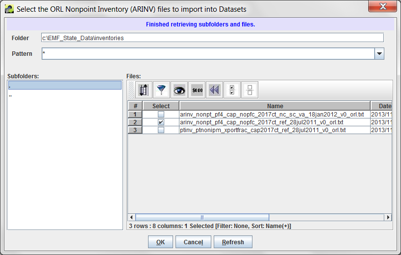
To use the remote file browser, you can navigate from your starting folder to the file by either typing or pasting a directory name into the Folder field or by using the Subfolders list on the left side of the window. In the Subfolders list, double-click on a folder’s name to go into that folder. If you need to go up a level, double-click the .. entry.
Once you reach the folder that contains your data files, select the files to import by clicking the checkbox next to each file’s name in the Files section of the browser. The Files section uses the Sort-Filter-Select Table described in Sec. 2.6.6 to list the files. If you have a large number of files in the directory, you can use the sorting and filtering options of the Sort-Filter-Select Table to help find the files you need.
You can also use the Pattern field in the remote file browser to only show files matching the entered pattern. By default the pattern is just the wildcard character * to match all files. Entering a pattern like arinv*2002*txt will match filenames that start with “arinv”, have “2002” somewhere in the filename, and then end with “txt”.
Once you’ve selected the files to import, click OK to save your selections and return to the Import Datasets dialog. The files you selected will be listed in the Filenames textbox in the Import Datasets dialog as shown in Fig. 3.33. If you selected a single file, the Dataset Names field will contain the filename of the selected file as the default dataset name.
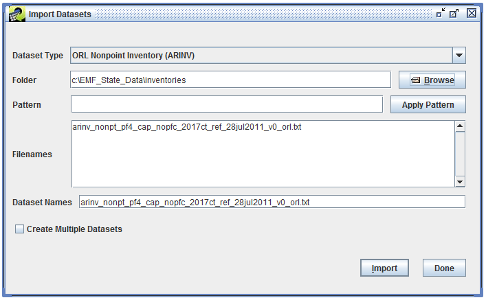
Update the Dataset Names field with your desired name for the dataset. If the dataset type has EXPORT_PREFIX or EXPORT_SUFFIX keywords assigned, these values will be automatically stripped from the dataset name. For example, the ORL Nonpoint Inventory (ARINV) dataset type defines EXPORT_PREFIX as “arinv_” and EXPORT_SUFFIX as “_orl.txt”. Suppose you select an ORL nonpoint inventory file named “arinv_nonpt_pf4_cap_nopfc_2017ct_ref_orl.txt” to import. By default the Dataset Names field in the Import Datasets dialog will be populated with “arinv_nonpt_pf4_cap_nopfc_2017ct_ref_orl.txt” (the filename). On import, the EMF will automatically convert the dataset name to “nonpt_pf4_cap_nopfc_2017ct_ref” removing the EXPORT_PREFIX and EXPORT_SUFFIX.
Click the Import button to start the dataset import. If there are any problems with your import settings, you’ll see a red error message displayed at the top of the Import Datasets window. Tbl. 3.13 shows some example error messages and suggested solutions.
| Example Error Message | Solution |
|---|---|
| A Dataset Type should be selected | Select a dataset type from the Dataset Type pull-down menu. |
| A Filename should be specified | Select a file to import. |
| A Dataset Name should be specified | Enter a dataset name in the Dataset Names textbox. |
| The ORL Nonpoint Inventory (ARINV) importer can use at most 1 files | You selected too many files to import for the dataset type. Select the correct number of files for the dataset type. If you want to import multiple files of the same dataset type, see Sec. 3.9.1. |
| The NIF3.0 Nonpoint Inventory importer requires at least 2 files | You didn’t select enough files to import for the dataset type. Select the correct number of files for the dataset type. |
| Dataset name nonpt_pf4_cap_nopfc_2017ct_ref has been used. | Each dataset in the EMF needs a unique dataset name. Update the dataset name to be unique. Remember that the EMF will automatically remove the EXPORT_PREFIX and EXPORT_SUFFIX if defined for the dataset type. |
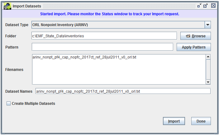
If your import settings are good, you will see the message “Started import. Please monitor the Status window to track your import request.” displayed at the top of the Import Datasets window as shown in Fig. 3.34.
In the Status window, you will see a status message like:
Started import of nonpt_pf4_cap_nopfc_2017ct_nc_sc_va_18jan2012_v0 [ORL Nonpoint Inventory (ARINV)] from arinv_nonpt_pf4_cap_nopfc_2017ct_nc_sc_va_18jan2012_v0.txt
Depending on the size of your file, the import can take a while to complete. Once the import is complete, you will see a status message like:
Completed import of nonpt_pf4_cap_nopfc_2017ct_nc_sc_va_18jan2012_v0 [ORL Nonpoint Inventory (ARINV)] in 57.6 seconds from arinv_nonpt_pf4_cap_nopfc_2017ct_nc_sc_va_18jan2012_v0.txt
To see your newly imported dataset, open the Dataset Manager window and find your dataset by dataset type or using the Advanced search. You may need to click the Refresh button in the upper right corner of the Dataset Manager window to get the latest dataset information from the EMF server.
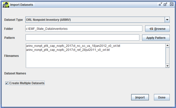
You can use the Import Datasets window to import multiple datasets of the same type at once. In the remote file browser (shown in Fig. 3.32), select all the files you would like to import and click OK. In the Import Datasets window, check the checkbox Create Multiple Datasets as shown in Fig. 3.35. The Dataset Names textbox goes away.
For each dataset, the EMF will automatically name the dataset using the corresponding filename. If the keywords EXPORT_PREFIX or EXPORT_SUFFIX are defined for the dataset type, the keyword values will be stripped from the filenames when generating the dataset names. If these keywords are not defined for the dataset type, then the dataset name will be identical to the filename.
Click the Import button to start importing the datasets. The Status window will display Started and Completed status messages for each dataset as it is imported.
Use a consistent naming scheme that works for your group. If you have a naming system already in place, continue using it in the EMF. You can enter your own dataset names when importing files and also edit a dataset’s name if you have the appropriate privileges. The EMF will automatically make sure that the dataset names are unique.
Avoid dates in your dataset names. When a dataset is exported, the EMF will automatically include the dataset’s last modified date in name of the exported file.
For monthly inventory files, include the three character month abbreviation in the dataset name (i.e. “jan”, “feb”, “mar”, etc.). These names are used in certain QA steps.
Enter as much metadata about each dataset as possible, for example the temporal resolution of the data, time period covered, and region. These fields can be used when filtering datasets in the Dataset Manager window.
Use the Project field to group sets of files together. EMF Administrators can create new project names to aid in organizing files.
Try out the different options for finding datasets in the Dataset Manager (Sec. 3.4) to see what works best for your workflow. You may find that the Advanced Dataset Search fits what you need to do or perhaps filtering the dataset list is more useful.
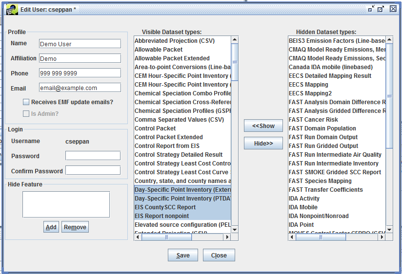
Hide dataset types that you don’t use. Each user can control the list of dataset types that the EMF client will use when displaying dataset type pull-down menus (like the Show Datasets of Type pull-down menu in the Manage Datasets window). From the Manage menu, select My Profile to show the Edit User window (Fig. 3.36). In this window, you can select dataset types from the Visible Dataset Types list, then click the Hide button to move the selected types to the Hidden Dataset Types list. Selecting items in the hidden list and clicking the Show button will move the selected types back to the visible list. Click the Save button to save your changes. Note that if the Dataset Manager window is open, you’ll need to close it and open it again for the list of dataset types to refresh.
The EMF allows you to perform various types of analyses on a dataset or set of datasets. For example, you can summarize the data by different aspects such as geographic region like county or state, SCC code, pollutant, or plant ID. You can also compare or sum multiple datasets. Within the EMF, running an analysis like this is called a QA step.
A dataset can have many QA steps associated with it. To view a dataset’s QA steps, first select the dataset in the Dataset Manager and click the Edit Properties button. Switch to the QA tab to see the list of QA steps as in Fig. 4.1.
At the bottom of the window you will see a row of buttons for interacting with the QA steps starting with Add from Template, Add Custom, Edit, etc. If you do not see these buttons, make sure that you are editing the dataset’s properties and not just viewing them.
Each dataset type can have predefined QA steps called QA Step Templates. QA step templates can be added to a dataset type and configured by EMF Administrators using the Dataset Type Manager (see Sec. 3.2). QA step templates are easy to run for a dataset because they’ve already been configured.
To see a list of available QA step templates for your dataset, open your dataset’s QA tab in the Dataset Properties Editor (Fig. 4.1). Click the Add from Template button to open the Add QA Steps dialog. Fig. 4.2 shows the available QA step templates for an ORL Nonroad Inventory.
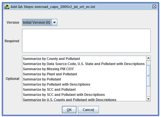
The ORL Nonroad Inventory has various QA step templates for generating different summaries of the inventory.
Summaries “with Descriptions” include more information than those without. For example, the results of the “Summarize by SCC and Pollutant with Descriptions” QA step will include the descriptions of the SCCs and pollutants. Because these summaries with descriptions need to retrieve data from additional tables, they are a bit slower to generate compared to summaries without descriptions.
Select a summary of interest (for example, Summarize by County and Pollutant) by clicking the QA step name. If your dataset has more than one version, you can choose which version to summarize using the Version pull-down menu at the top of the window. Click OK to add the QA step to the dataset.
The newly added QA step is now shown in the list of QA steps for the dataset (Fig. 4.3).
To see the details of the QA step, select the step and click the Edit button. This brings up the Edit QA Step window like Fig. 4.4.
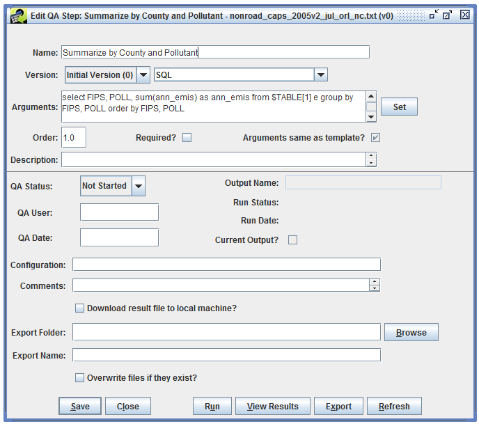
The QA step name is shown at the top of the window. This name was automatically set by the QA step template. You can edit this name if needed to distinguish this step from other QA steps.
The Version pull-down menu shows which version of the data this QA step will run on.
The pull-down menu to the right of the Version setting indicates what type of program will be used for this QA step. In this case, the program type is “SQL” indicating that the results of this QA step will be generated using a SQL query. Most of the summary QA steps are generated using SQL queries. The EMF allows other types of programs to be run as QA steps including Python scripts and various built-in analyses like converting average-day emissions to an annual inventory.
The Arguments textbox shows the arguments used by the QA step program. In this case, the QA step is a SQL query and the Arguments field shows the query that will be run. The special SQL syntax used for QA steps is discussed in Sec. 4.10.
Other items of interest in the Edit QA Step window include the description and comment textboxes where you can enter a description of your QA step and any comments you have about running the step.
The QA Status field shows the overall status of the QA step. Right now the step is listed as “Not Started” because it hasn’t been run yet. Once the step has been run, the status will automatically change to “In Progress”. After you’ve reviewed the results, you can mark the step as “Complete” for future reference.
The Edit QA Step window also includes options for exporting the results of a QA step to a file. This is described in Sec. 4.5.
At this point, the next step is to actually run the QA step as described in Sec. 4.4.
In addition to using QA steps from templates, you can define your own custom QA steps. From the QA tab of the Dataset Properties Editor (Fig. 4.1), click the Add Custom button to bring up the Add Custom QA Step dialog as shown in Fig. 4.5.
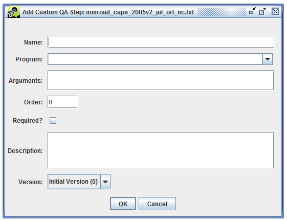
In this dialog, you can configure your custom QA step by entering its name, the program to use, and the program’s arguments.
Creating a custom QA step from scratch is an advanced feature. Oftentimes, you can start by copying an existing step and tweaking it through the Edit QA Step interface.
Sec. 4.7 shows how to create a custom QA step that uses the built-in QA program “Average day to Annual Inventory” to calculate annual emissions from average-day emissions. Sec. 4.8 demonstrates using the Compare Datasets QA program to compare two inventories. Sec. 4.9 gives an example of creating a custom QA step based on a SQL query from an existing QA step.
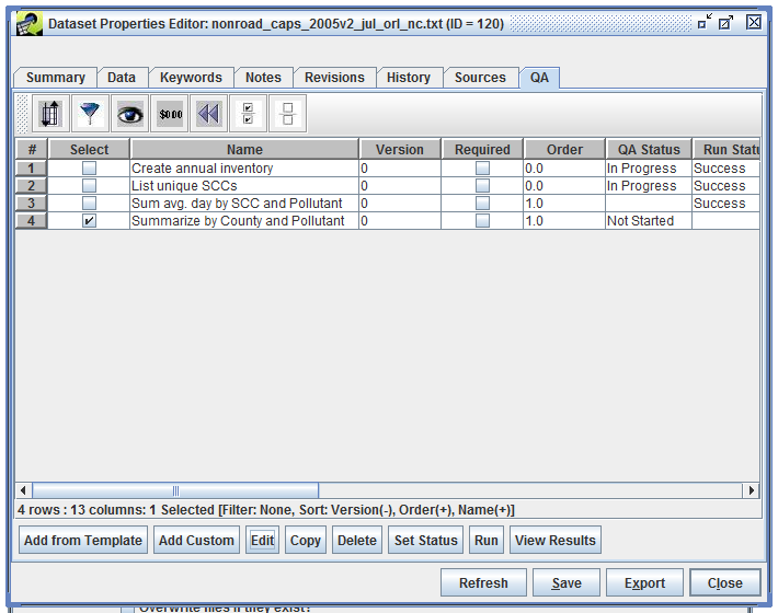
To run a QA step, open the QA tab of the Dataset Properties Editor and select the QA step you want to run as shown in Fig. 4.6.
Click the Run button at the bottom of the window to run the QA step. You can also run a QA step from the Edit QA Step window. The Status window will display messages when the QA step begins running and when it completes:
Started running QA step ‘Summarize by County and Pollutant’ for Version ‘Initial Version’ of Dataset ‘nonroad_caps_2005v2_jul_orl_nc.txt’
Completed running QA step ‘Summarize by County and Pollutant’ for Version ‘Initial Version’ of Dataset ‘nonroad_caps_2005v2_jul_orl_nc.txt’
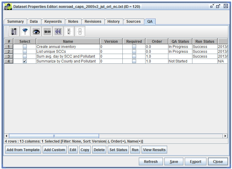
In the QA tab, click the Refresh button to update the table of QA steps as shown in Fig. 4.7.
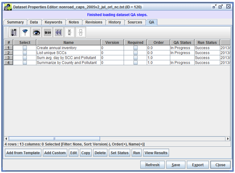
The overall QA step status (the QA Status column) has changed from “Not Started” to “In Progress” and the Run Status is now “Success”. The list of QA steps also shows the time the QA step was run in the When column.
To view the results of the QA step, select the step in the QA tab and click the View Results button. A dialog like Fig. 4.8 will pop-up asking how many records of the results you would like to preview.
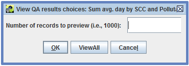
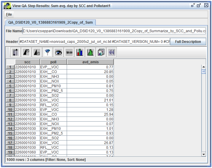
Enter the number of records to view or click the View All button to see all records. The View QA Step Results window will display the results of the QA step as shown in Fig. 4.9.
In addition to viewing the results of a QA step in the EMF client application, you can export the results as a comma-separated values (CSV) file. CSV files can be directly opened by Microsoft Excel or other spreadsheet programs to make charts or for further analysis.
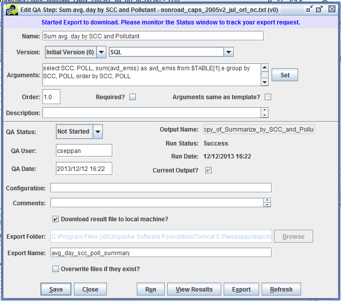
To export the results of a QA step, select the QA step of interest in the QA tab of the Dataset Properties Editor. Then click the Edit button to bring up the Edit QA Step window as shown in Fig. 4.10.
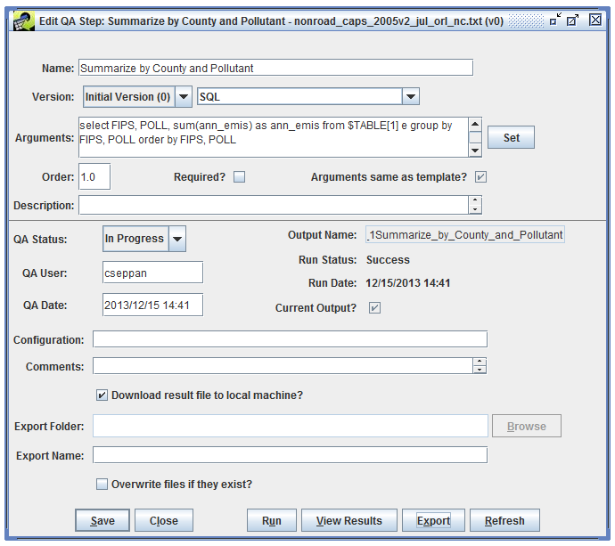
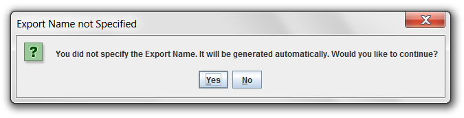
Typically, you will want to check the Download result file to local machine? checkbox so the exported file will automatically be downloaded to your local machine. You can type in a name for the exported file in the Export Name field. Then click the Export button. If you did not enter an Export Name, the application will confirm that you want to use an auto-generated name with the dialog shown in Fig. 4.11.
Next, you’ll see the Export QA Step Results customization window (Fig. 4.12).
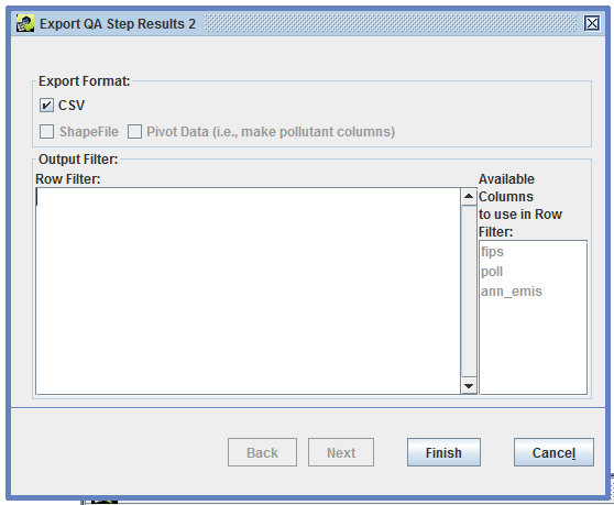
The Row Filter textbox allows you to limit which rows of the QA step results to include in the exported file. Tbl. 3.11 provides some examples of the syntax used by the row filter. Available Columns lists the column names from the results that could be used in a row filter. In Fig. 4.12, the columns fips, poll, and ann_emis are available. To export only the results for counties in North Carolina (state FIPS code = 37), the row filter would be fips like '37%'.
Click the Finish button to start the export. At the top of the Edit QA Step window, you’ll see the message “Started Export. Please monitor the Status window to track your export request.” like Fig. 4.13
Once your export is complete, you will see a message in the Status window like
Completed exporting QA step ‘Summarize by SCC and Pollutant’ for Version ‘Initial Version’ of Dataset ‘nonpt_pf4_cap_nopfc_2017ct_nc_sc_va’ to <server directory>avg_day_scc_poll_summary.csv. The file will start downloading momentarily, see the Download Manager for the download status.
You can bring up the Downloads window as shown in Fig. 4.14 by opening the Window menu at the top of the EMF main window and selecting Downloads.
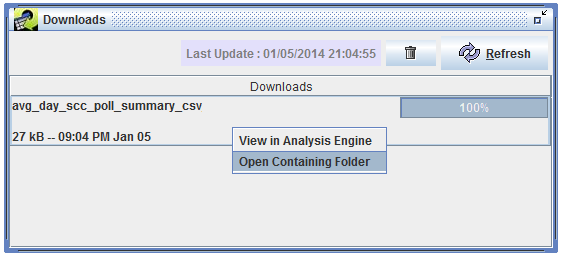
As your file is downloading, the progress bar on the right side of the window will update to show you the progress of the download. Once it reaches 100%, your download is complete. Right click on the filename in the Downloads window and select Open Containing Folder to open the folder where the file was downloaded.
If you have Microsoft Excel or another spreadsheet program installed, you can double-click the downloaded CSV file to open it.
QA step results that include latitude and longitude information can be mapped with geographic information systems (GIS), mapping tools, and Google Earth. Many summaries that have “with Descriptions” in their names include latitude and longitude values. For plant-level summaries, the latitude and longitude in the output are the average of all the values for the specific combination of FIPS and plant ID. For county- and state-level summaries, the latitude and longitude are the centroid values specified in the “fips” table of the EMF reference schema.
To export a KMZ file that can be loaded into Google Earth, you will first need to view the results of the QA step. You can view a QA step’s results by either selecting the QA step in the QA tab of the Dataset Properties Editor (see Fig. 4.1) and then clicking the View Results button, or you can click View Results from the Edit QA Step window. Fig. 4.15 shows the View QA Step Results window for a summary by county and pollutant with descriptions. The summary includes latitude and longitude values for each county.
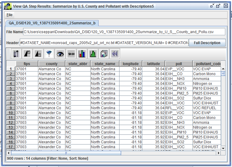
From the File menu in the top left corner of the View QA Step Results window, select Google Earth. Make sure to look at the File menu for the View QA Step Results window, not the main EMF application. The Create Google Earth file window will be displayed as shown in Fig. 4.16.
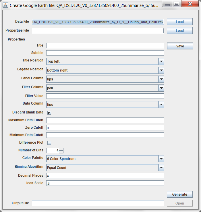
In the Create Google Earth file window, the Label Column pull-down menu allows you to select which column will be used to label the points in the KMZ file. This label will appear when you mouse over a point in Google Earth. For a plant summary, this would typically be “plant_name”; county or state summaries would use “county” or “state_name” respectively.
If your summary has data for multiple pollutants, you will often want to specify a filter so that data for only one pollutant is included in the KMZ file. To do this, specify a Filter Column (e.g. “poll”) and then type in a Filter Value (e.g. "EVP__VOC").
The Data Column pull-down menu specifies the column to use for the value displayed when you mouse over a point in Google Earth such as annual emissions (“ann_emis”). The mouse over information will have the form: <value from Label Column> : <value from Data Column>.
The Maximum Data Cutoff and Minimum Data Cutoff fields allow you to exclude data points above or below certain thresholds.
If you want to control the size of the points, you can adjust the value of the Icon Scale setting between 0 and 1. The default setting is 0.3; values smaller than 0.3 result in smaller circles and values larger than 0.3 will result in larger circles.
Tooltips are available for all of the settings in the Create Google Earth file window by mousing over each field.
Once you have specified your settings, click the Generate button to create the KMZ file. The location of the generated file is shown in the Output File field. If your computer has Google Earth installed, you can click the Open button to open the file in Google Earth.
If you find that you need to repeatedly create similar KMZ files, you can save your settings to a file by clicking the Save button. The next time you need to generate a Google Earth file, click the Load button next to the Properties File field to load your saved settings.
In addition to analyzing individual datasets, the EMF can run QA steps that use multiple datasets. In this section, we’ll show how to create a custom QA step that calculates an annual inventory from 12 month-specific average-day emissions inventories.
To get started, we’ll need to select a dataset to associate the QA step with. As a best practice, add the QA step to the January-specific dataset in the set of 12 month-specific files. This isn’t required by the EMF but it can make finding multi-file QA steps easier later on. If you have more than 12 month-specific files to use (e.g. 12 non-California inventories and 12 California inventories), add the QA step to the “main” January inventory file (e.g. the non-California dataset).
After determining which dataset to add the QA step to, create a new custom QA step as described in Sec. 4.3. Fig. 4.17 shows the Add Custom QA Step dialog. We’ve entered a name for the step and used the Program pull-down menu to select “Average day to Annual Inventory”.
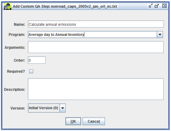
“Average day to Annual Inventory” is a QA program built into the EMF that takes a set of average-day emissions inventories as input and outputs an annual inventory by calculating monthly total emissions and summing all months. Click the OK button in the Add Custom QA Step dialog to save the new QA step. We’ll enter the QA program arguments in a minute. Back in the QA tab of the Dataset Properties Editor, select the newly created QA step and click Edit to open the Edit QA Step window shown in Fig. 4.18.
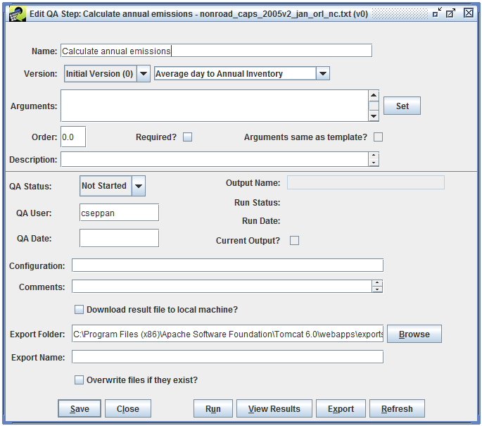
We need to define the arguments that will be sent to the QA program that this QA step will run. The QA program is “Average day to Annual Inventory” so the arguments will be a list of month-specific inventories. Click the Set button to the right of the Arguments box to open the Set Inventories dialog as shown in Fig. 4.19.
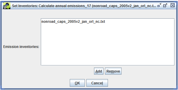
The Set Inventories dialog is specific to the “Average day to Annual Inventory” QA program. Other QA programs have different dialogs for setting up their arguments. The January inventory that we added the QA step to is already listed. We need to add the other 11 month-specific inventory files. Click the Add button to open the Select Datasets dialog shown in Fig. 4.20.
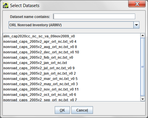
In the Select Datasets dialog, the dataset type is automatically set to ORL Nonroad Inventory (ARINV) matching our January inventory. The other ORL nonroad inventory datasets are shown in a list. We can use the Dataset name contains: field to enter a search term to narrow the list. We’re using 2005 inventories so we’ll enter 2005 as our search term to match only those datasets whose name contains “2005”. Then we’ll select all the inventories in the list as shown in Fig. 4.21.
Select inventories by clicking on the dataset name. You can select a range of datasets by clicking on the first dataset you want to select in the list. Then hold down the Shift key while clicking on the last dataset you want to select. All of the datasets in between will also be selected. If you hold down the Ctrl key while clicking on datasets, you can select multiple items from the list that aren’t next to each other.
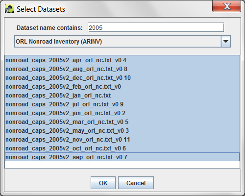
Click the OK button in the Select Datasets dialog to save the selected inventories and return to the Set Inventories dialog. As shown in Fig. 4.22, the list of emission inventories now contains all 12 month-specific datasets.
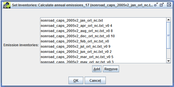
Click the OK button in the Set Inventories dialog to return to the Edit QA Step window shown in Fig. 4.23. The Arguments textbox now lists the 12 month-specific inventories and the flag (-inventories) needed for the “Average day to Annual Inventory” QA program.
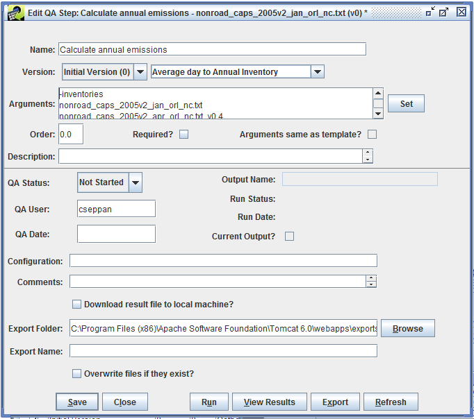
Click the Save button at the bottom of the Edit QA Step window to save the QA step. This QA step can now be run as described in Sec. 4.4.
The Compare Datasets QA program allows you to aggregate and compare datasets using a variety of grouping options. You can compare datasets with the same dataset type or different types. In this section, we’ll set up a QA step to compare the average day emissions from two ORL nonroad inventories by SCC and pollutant.
First, we’ll select a dataset to associate the QA step with. In this example, we’ll be comparing January and February emissions using the January dataset as the base inventory. The EMF doesn’t dictate which dataset should have the QA step associated with it so we’ll choose the base dataset as a convention. From the Dataset Manager, select the January inventory (shown in Fig. 4.24) and click the Edit Properties button.
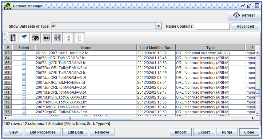
Open the QA tab (shown in Fig. 4.25) and click Add Custom to add a new QA step.
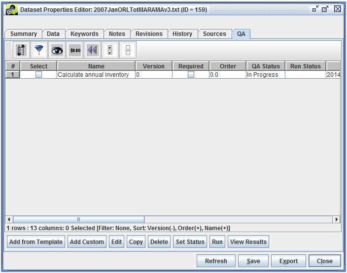
In the Add Custom QA Step dialog shown in Fig. 4.26, enter a name for the new QA step like “Compare to February”. Use the Program pull-down menu to select the QA program “Compare Datasets”.
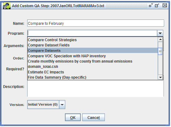
You can enter a description of the QA step as shown in Fig. 4.27. Then click OK to save the QA step. We’ll be setting up the arguments to the Compare Datasets QA program in just a minute.
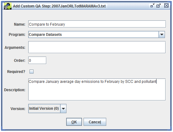
Back in the QA tab of the Dataset Properties Editor, select the newly created QA step and click the Edit button (see Fig. 4.28).
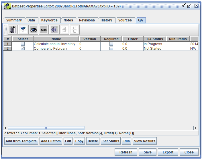
In the Edit QA Step window (shown in Fig. 4.29), click the Set button to the right of the Arguments textbox.
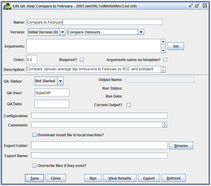
A custom dialog is displayed (Fig. 4.30) to help you set up the arguments needed by the Compare Datasets QA program.
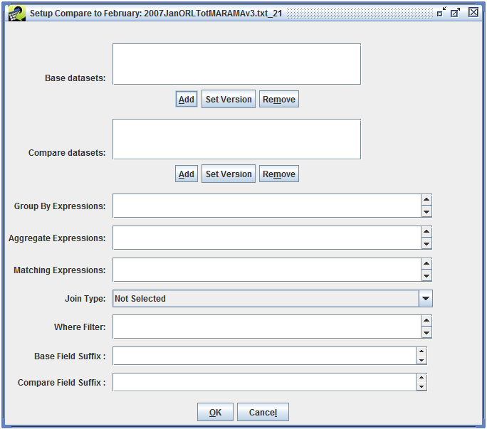
To get started, we’ll set the base datasets. Click the Add button underneath the Base Datasets area to bring up the Select Datasets dialog shown in Fig. 4.31.
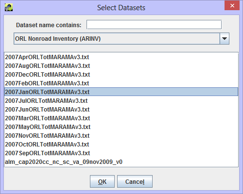
Select one or more datasets to use as the base datasets in the comparison. For this example, we’ll select the January inventory by clicking on the dataset name. Then click OK to close the dialog and return to the setup dialog. The setup dialog now shows the selected base dataset as in Fig. 4.32.
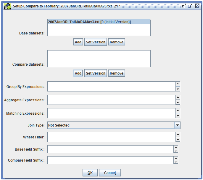
Next, we’ll add the dataset we want to compare against by clicking the Add button underneath the Compare Datasets area. The Select Datasets dialog is displayed like in Fig. 4.33. We’ll select the February inventory and click the OK button.
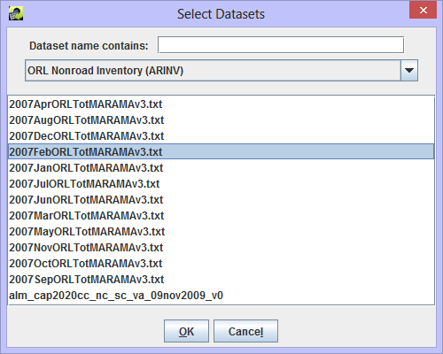
Returning to the setup dialog, the comparison dataset is now set as shown in Fig. 4.34.
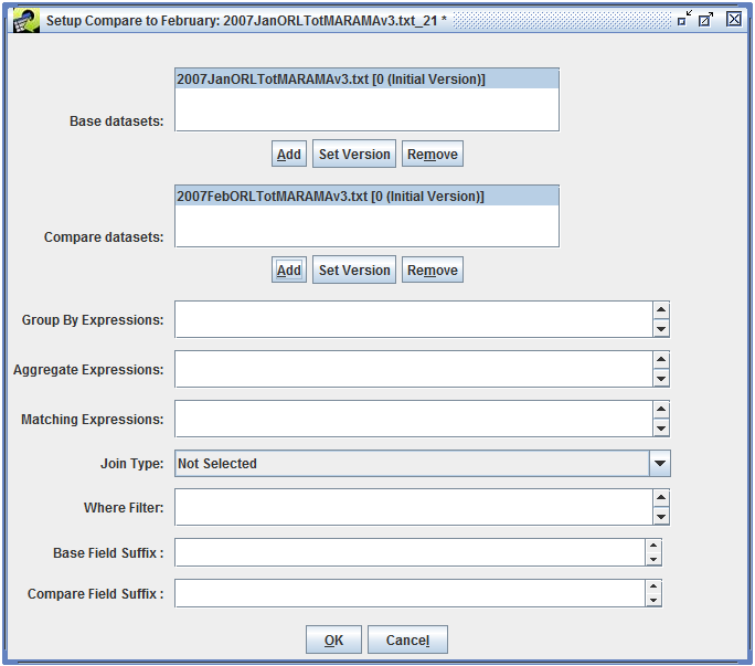
The list of base and comparison datasets includes which version of the data will be used in the QA step. For example, the base dataset 2007JanORLTotMARAMAv3.txt [0 (Initial Version)] indicates that version 0 (named “Initial Version”) will be used. When you select the base and comparison datasets, the EMF automatically uses each dataset’s Default Version. If any of the datasets have a different version that you would like to use for the QA step, select the dataset name and then click the Set Version button underneath the selected dataset. The Set Version dialog shown in Fig. 4.35 lets you pick which version of the dataset you would like to use.
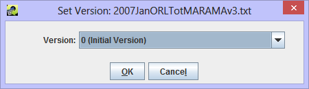
Next, we need to tell the Compare Datasets QA program how to compare the two datasets. We’re going to sum the average-day emissions in each dataset by SCC and pollutant and then compare the results from January to February. In the ORL Nonroad Inventory dataset type, the SCCs are stored in a field called scc, the pollutant codes are stored in a column named poll, and the average-day emissions are stored in a field called avd_emis. In the Group By Expressions textbox, type scc, press Enter, and then type poll. In the Aggregate Expressions textbox, type avd_emis. Fig. 4.36 shows the setup dialog with the arguments entered.
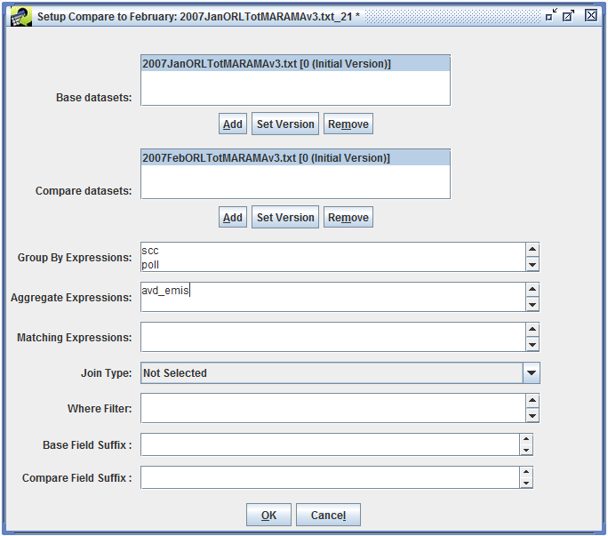
In this example, we’re comparing two datasets of the same type (ORL Nonroad Inventory). This means that the data field names will be consistent between the base and comparison datasets. When you compare datasets with different types, the field names might not match. The Matching Expressions textbox allows you to define how the fields from the base dataset should be matched to the comparison dataset. For this case, we don’t need to enter anything in the Matching Expressions textbox or any of the remaining fields in the setup dialog. The Compare Datasets arguments are described in more detail in Sec. 4.8.1.
In the setup dialog, click OK to save the arguments and return to the Edit QA Step window. The Arguments textbox now lists the arguments that we set up in the previous step (see Fig. 4.37).
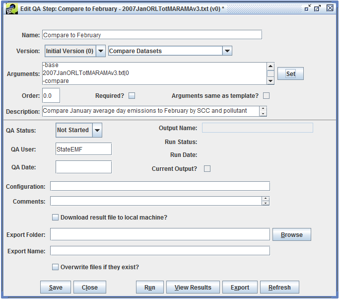
The QA step is now ready to run. Click the Run button to start running the QA step. A message is displayed at the top of the window as shown in Fig. 4.38.
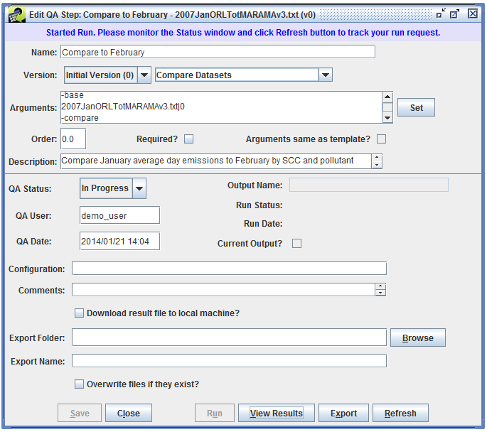
In the Status window, you’ll see a message about starting to run the QA step followed by a completion message once the QA step has finished running. Fig. 4.39 shows the two status messages.
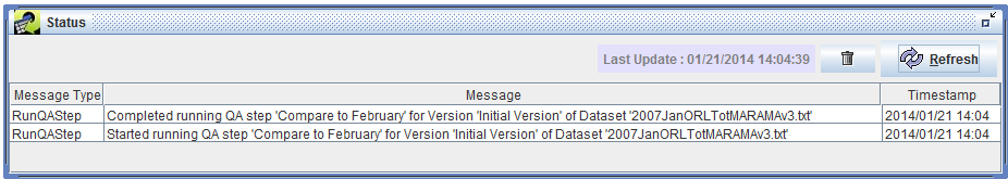
Once the status message
Completed running QA step ‘Compare to February’ for Version ‘Initial Version’ of Dataset ‘2007JanORLTotMARAMAv3.txt’
is displayed, the QA step has finished running. In the Edit QA Step window, click the Refresh button to display the latest information about the QA step. The fields Run Status and Run Date will be populated with the latest run information as shown in Fig. 4.40.
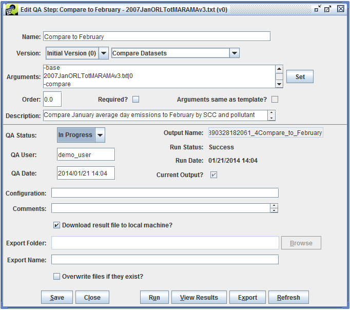
Now, we can view the QA step results or export the results. First, we’ll view the results inside the EMF client. Click the View Results button to open the View QA Step Results window as shown in Fig. 4.41.
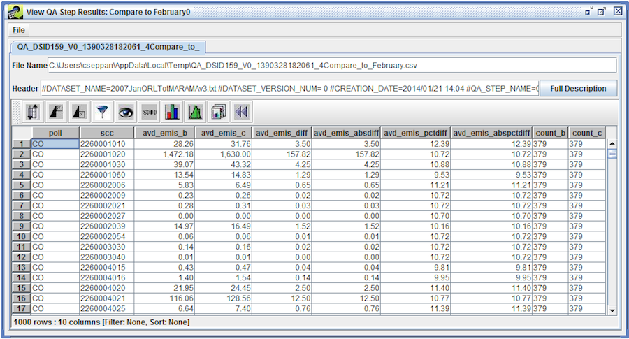
Tbl. 4.1 describes each column in the QA step results.
| Column Name | Description |
|---|---|
poll |
Pollutant code |
scc |
SCC code |
avd_emis_b |
Summed average-day emissions from base dataset (January) for this pollutant and SCC |
avd_emis_c |
Summed average-day emissions from comparison dataset (February) for this pollutant and SCC |
avd_emis_diff |
avd_emis_c - avd_emis_b |
avd_emis_absdiff |
Absolute value of avd_emis_diff |
avd_emis_pctdiff |
100 * (avd_emis_diff / avd_emis_b) |
avd_emis_abspctdiff |
Absolute value of avd_emis_pctdiff |
count_b |
Number of records from base dataset included in this row’s results |
count_c |
Number of records from comparison dataset included in this row’s results |
To export the QA step results, return to the Edit QA Step window as shown in Fig. 4.42. Select the checkbox labeled Download result file to local machine?. In this example, we have entered an optional Export Name for the output file. If you don’t enter an Export Name, the output file will use an auto-generated name. Click the Export button.
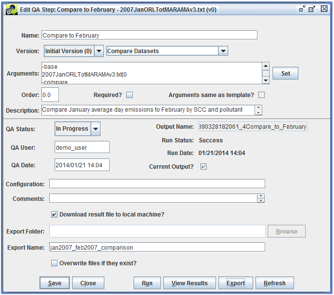
The Export QA Step Results dialog will be displayed as shown in Fig. 4.43. For more information about the Row Filter option, see Sec. 4.5. To export all the result records, click the Finish button.
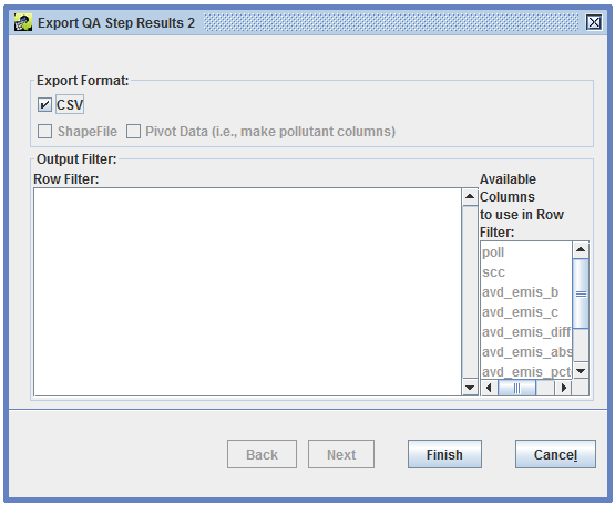
Back in the Edit QA Step window, a message is displayed at the top of the window indicating that the export has started. See Fig. 4.44.
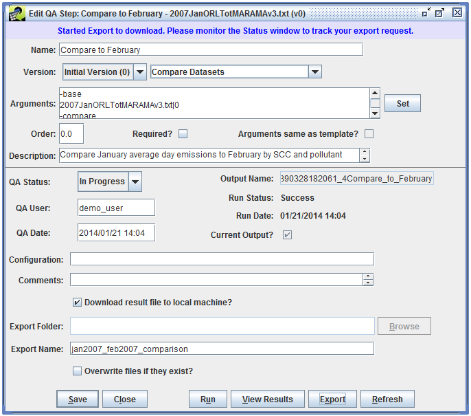
Check the Status window to see the status of the export as shown in Fig. 4.45.
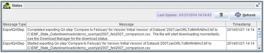
Once the export is complete, the file will start downloading to your computer. Open the Downloads window to check the download status. Once the progress bar reaches 100%, the download is complete. Right click on the results file and select Open Containing Folder as shown in Fig. 4.46.
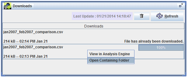
Fig. 4.47 shows the downloaded file in Windows Explorer. By default, files are downloaded to a temporary directory on your computer. Some disk cleanup programs can automatically delete files in temporary directories; you should move any downloads you want to keep to a more permanent location on your computer.
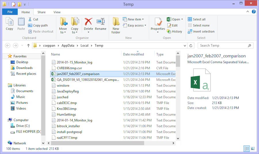
The downloaded file is a CSV (comma-separated values) file which can be opened in Microsoft Excel or other spreadsheet programs. Double-click the filename to open the file. Fig. 4.48 shows the QA step results in Microsoft Excel.
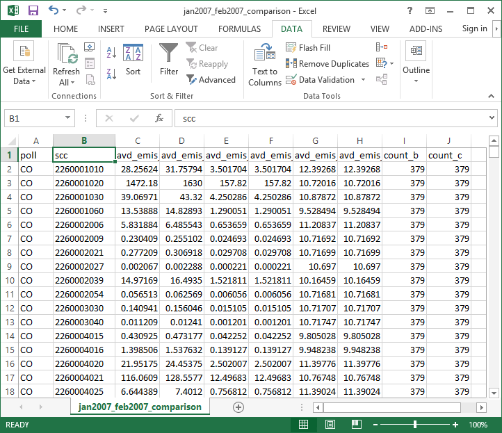
The Group By Expressions are a list of columns/expressions that are used to group the dataset records for aggregation. The expressions must contain valid columns from either the base or comparison datasets. If a column exists only in the base or compare dataset, then a Matching Expression must be specified in order for a proper mapping to happen during the comparison analysis. A group by expression can be aliased by adding the AS <alias> clause to the expression; this alias is used as the column name in the QA step results. A group by expression can also contain SQL functions such as substring or string concatenation using ||.
Sample Group By Expressions
scc AS scc_code
substring(fips, 1, 2) as fipsst
or
fipsst||fipscounty as fips
substring(scc, 1, 5) as scc_lv5
The Aggregate Expressions are a list of columns/expressions that will be aggregated (summed) using the specified group by expressions. The expressions must contain valid columns from either the base or comparison datasets. If a column exists only in the base or compare dataset, then a Matching Expression must be specified in order for a proper mapping to happen during the comparison analysis.
Sample Aggregate Expressions
ann_emis
avd_emis
The Matching Expressions are a list of expressions used to match base dataset columns/expressions to comparison dataset columns/expressions. A matching expression consists of three parts: the base dataset expression, the equals sign, and the comparison dataset expression (i.e. base_expression=comparison_expression).
Sample Matching Expressions
substring(fips, 1, 2)=substring(region_cd, 1, 2)
scc=scc_code
ann_emis=emis_ann
avd_emis=emis_avd
fips=fipsst||fipscountyThe Join Type specifies which type of SQL join should be used when performing the comparison.
| Join Type | Description |
|---|---|
| INNER JOIN | Only include rows that exist in both the base and compare datasets based on the group by expressions |
| LEFT OUTER JOIN | Include all rows from the base dataset, only include rows from the compare dataset that meet the group by expressions |
| RIGHT OUTER JOIN | Include all rows from the compare dataset, only include rows from the base dataset that meet the group by expressions |
| FULL OUTER JOIN | Include all rows from both the base and compare datasets |
The default join type is FULL OUTER JOIN.
The Where Filter is a SQL WHERE clause that is used to filter both the base and comparison datasets. The expressions in the WHERE clause must contain valid columns from either the base or comparison datasets. If a column exists only in the base or compare dataset, then a Matching Expression must be specified in order for a proper mapping to happen during the comparison analysis.
Sample Row Filter
substring(fips, 1, 2) = '37' and SCC_code in ('10100202', '10100203')
or
fips like '37%' and SCC_code like '101002%'
The Base Field Suffix is appended to the base aggregate expression name that is returned in the output. For example, an Aggregate Expression ann_emis with a Base Field Suffix 2005 will be returned as ann_emis_2005 in the QA step results.
The Compare Field Suffix is appended to the comparison aggregate expression name that is returned in the output. For example, an Aggregate Expression ann_emis with a Compare Field Suffix 2008 will be returned as ann_emis_2008 in the QA step results.
Fig. 4.49 shows the setup dialog for the following example of the Compare Datasets QA program. We are setting up a plant level comparison of a set of two inventories (EGU and non-EGU) versus another set of two inventories (EGU and non-EGU). All four inventories are the same dataset type. The annual emissions will be grouped by FIPS code, plant ID, and pollutant. There is no mapping required because the dataset types are identical; the columns fips, plantid, poll, and ann_emis exist in both sets of datasets. This comparison is limited to the state of North Carolina via the Where Filter:
substring(fips, 1, 2)='37'The QA step results will have columns named ann_emis_base, ann_emis_compare, count_base, and count_compare using the Base Field Suffix and Compare Field Suffix.
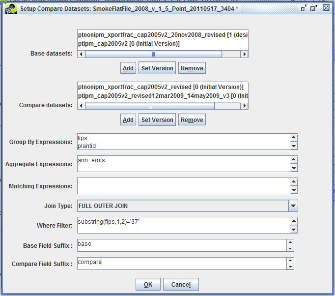
Fig. 4.50 shows the setup dialog for a second example of the Compare Datasets QA program. This example takes a set of ORL nonpoint datasets and compares it to a single FF10 nonpoint inventory. We are grouping by state (first two digits of the FIPS code) and pollutant. A mapping expression is needed between the ORL column fips and the FF10 column region_cd:
substring(fips, 1, 2)=substring(region_cd, 1, 2)Another mapping expression is needed between the columns ann_emis and ann_value:
ann_emis=ann_valueNo mapping is needed for pollutant because both dataset types use the same column name poll. This comparison is limited to three states and to sources that have annual emissions greater than 1000 tons. These constraints are specified via the Where Filter:
substring(fips, 1, 2) in ('37','45','51') and ann_emis > 1000In the QA step results, the base dataset column will be named ann_emis_2002 and the compare dataset column will be named ann_emis_2008.
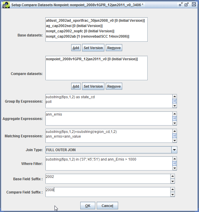
Suppose you have an ORL nonroad inventory that contains average-day emissions instead of annual emissions. The QA step templates that can generate inventory summaries report summed annual emissions. If you want to get a report of the average-day emissions, you can create a custom SQL QA step.
First, let’s look at the structure of a SQL QA step created from a QA step template. Fig. 4.51 shows a QA step that generates a summary of the annual emissions by county and pollutant.
This QA step uses a custom SQL query shown in the Arguments textbox:
select FIPS, POLL, sum(ann_emis) as ann_emis from $TABLE[1] e group by FIPS, POLL order by FIPS, POLLFor the ORL nonroad inventory dataset type, the annual emission values are stored in a database column named ann_emis while the average-day emissions are in a column named avd_emis. For any dataset you can see the names of the underlying data columns by viewing the raw data as described in Sec. 3.6.
To create an average-day emissions report, we’ll need to switch ann_emis in the above SQL query to avd_emis. In addition, the annual emissions report sums the emissions across the counties and pollutants. For average-day emissions, it might make more sense to compute the average emissions by county and pollutant. In the SQL query we can change sum(ann_emis) to avg(avd_emis) to call the SQL function which computes averages.
Our final revised SQL query is
select FIPS, POLL, avg(avd_emis) as avd_emis from $TABLE[1] e group by FIPS, POLL order by FIPS, POLLOnce we know what SQL query to run, we’ll create a custom QA step. Sec. 4.3 describes how to add a custom QA step to a dataset. Fig. 4.52 shows the new custom QA step with a name assigned and the Program pull-down menu set to SQL so that the custom QA step will run a SQL query. Our custom SQL query is pasted into the Arguments textbox.
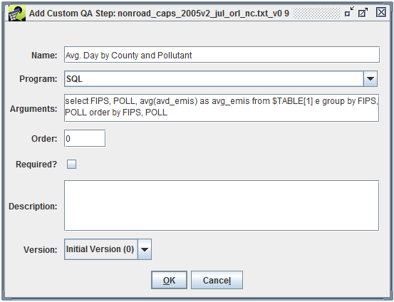
Click the OK button to save the QA step. The newly added QA step is now shown in the list of QA steps for the dataset (Fig. 4.53).
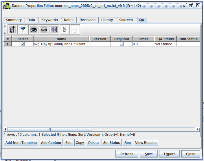
At this point, you can run the QA step as described in Sec. 4.4 and view and export the QA step results (Sec. 4.5) just like any other QA step.
What if our custom SQL had a typo? Suppose we accidently entered the average-day emissions column name as avg_emis instead of avd_emis. When the QA step is run, it will fail to complete successfully. The Status window will display a message like
Failed to run QA step Avg. Day by County and Pollutant for Version ‘Initial Version’ of Dataset <dataset name>. Check the query -ERROR: column “avg_emis” does not exist
Other types of SQL errors will be displayed in the Status window as well. If the SQL query uses an invalid function name like average(avd_emis) instead of avg(avd_emis), the Status window message is
Failed to run QA step Avg. Day by County and Pollutant for Version ‘Initial Version’ of Dataset <dataset name>. Check the query -ERROR: function average(double precision) does not exist
Each of the QA steps that create summaries use a customized SQL syntax that is very similar to standard SQL, except that it includes some EMF-specific concepts that allow the queries to be defined generally and then applied to specific datasets as needed. For example, the EMF syntax for the “Summarize by SCC and Pollutant” query is:
select SCC, POLL, sum(ann_emis) as ann_emis from $TABLE[1] e group by SCC, POLL order by SCC, POLLThe only difference between this and standard SQL is the use of the $TABLE[1] syntax. When this query is run, the $TABLE[1] portion of the query is replaced with the table name that contains the dataset’s data in the EMF database. Most datasets have their own tables in the EMF schema, so you do not normally need to worry about selecting only the records for the specific dataset of interest. The customized syntax also has extensions to refer to another dataset and to refer to specific versions of other datasets using tokens other than $TABLE. For the purposes of this discussion, it is sufficient to note that these other extensions exist.
Some of the summaries are constructed using more complex queries that join information from other tables, such as the SCC and pollutant descriptions, and to account for any missing descriptions. For example, the syntax for the “Summarize by SCC and Pollutant with Descriptions” query is:
select e.SCC,
       coalesce(s.scc_description,'AN UNSPECIFIED DESCRIPTION')::character varying(248) as scc_description,
       e.POLL,
       coalesce(p.descrptn,'AN UNSPECIFIED DESCRIPTION')::character varying(11) as pollutant_code_desc,
       coalesce(p.name,'AN UNSPECIFIED SMOKE NAME')::character varying(11) as smoke_name,
       p.factor,
       p.voctog,
       p.species,
       coalesce(sum(ann_emis), 0) as ann_emis,
       coalesce(sum(avd_emis), 0) as avd_emis
from $TABLE[1] e
left outer join reference.invtable p on e.POLL=p.cas
left outer join reference.scc s on e.SCC=s.scc
group by e.SCC,e.POLL,p.descrptn,s.scc_description,p.name,p.factor,p.voctog,p.species
order by e.SCC, p.name
This query is quite a bit more complex, but is still supported by the EMF QA step processing system.
In the EMF, cases are used to organize data and settings needed for model runs. For example, a case might run MOVES2014 to generate emission factors for a set of reference counties, or a case may run SMOKE to create inputs for CMAQ. Cases are a flexible concept to accommodate many different types of processing. Cases are organized into:
When a job is run, it can produce messages that are stored as the history for the job. A job may also produce data files that are automatically imported into the EMF; these datasets are referred to as outputs for the job.
To work with cases in the EMF, select the Manage menu and then Cases. This opens the Case Manager window, which will initially be empty as shown in Fig. 5.1.
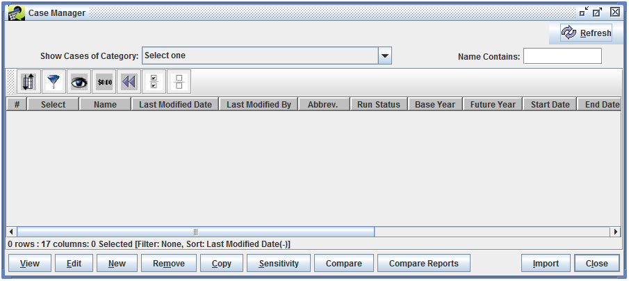
To show all cases currently in the EMF, use the Show Cases of Category pull-down to select All. The Case Manager window will then list all the cases as shown in Fig. 5.2.
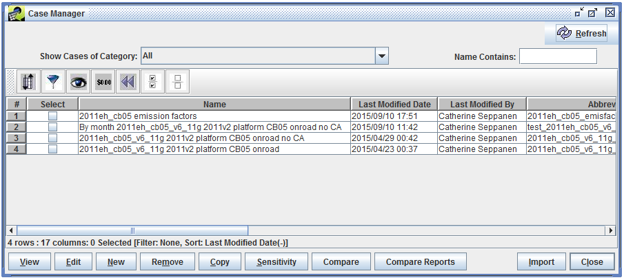
The Case Manager window shows a summary of each case. Tbl. 5.1 lists each column in the window. Many of the values are optional and may or may not be used depending on the specific model and type of case.
| Column | Description |
|---|---|
| Name | The unique name for the case. |
| Last Modified Date | The most recent date and time when the case was modified. |
| Last Modified By | The user who last modified the case. |
| Abbrev. | The unique abbreviation assigned to the case. |
| Run Status | The overall run status of the case. Values are Not Started, Running, Failed, and Complete. |
| Base Year | The base year of the case. |
| Future Year | The future year of the case. |
| Start Date | The starting date and time of the case. |
| End Date | The ending date and time of the case. |
| Regions | A list of modeling regions assigned to the case. |
| Model to Run | The model that the case will run. |
| Downstream | The model that the case is creating output for. |
| Speciation | The speciation mechanism used by the case. |
| Category | The category assigned to the case. |
| Project | The project assigned to the case. |
| Is Final | Indicates if the case has been marked as final. |
In the Case Manager window, the Name Contains textbox can be used to quickly find cases by name. The search term is not case sensitive and the wildcard character * (asterisk) can be used in the search.
To work with a case, select the case by checking the checkbox in the Select column, then click the desired action button in the bottom of the window. Tbl. 5.2 describes each button.
| Command | Description |
|---|---|
| View | Opens the Case Viewer window to view the details of the case in read-only mode. |
| Edit | Opens the Case Editor window to edit the details of the case. |
| New | Opens the Create a Case window to start creating a new case. |
| Remove | Removes the selected case; a prompt is displayed confirming the deletion. |
| Copy | Copies the selected case to a new case named “Copy of case name”. |
| Sensitivity | Opens the sensitivity tool, used to make emissions adjustments to existing SMOKE cases. |
| Compare | Generates a report listing the details of two or more cases and whether the settings match. |
| Compare Reports | Opens the Compare Case window which can be used to compare the outputs from different cases. |
| Import | Opens the Import Cases window where case information that was previously exported from the EMF can be imported from text files. |
| Close | Closes the Case Manager window. |
| Refresh | Refreshes the list of cases and information about each case. (This button is in the top right corner of the Case Manager window.) |
To view or edit the details of a case, select the case in the Case Manager window, then click the View or Edit button. Fig. 5.3 shows the Case Viewer window, while Fig. 5.4 shows the Case Editor window for the same case. Data in the Case Viewer window is not editable, and the Case Viewer window does not have a Save button.
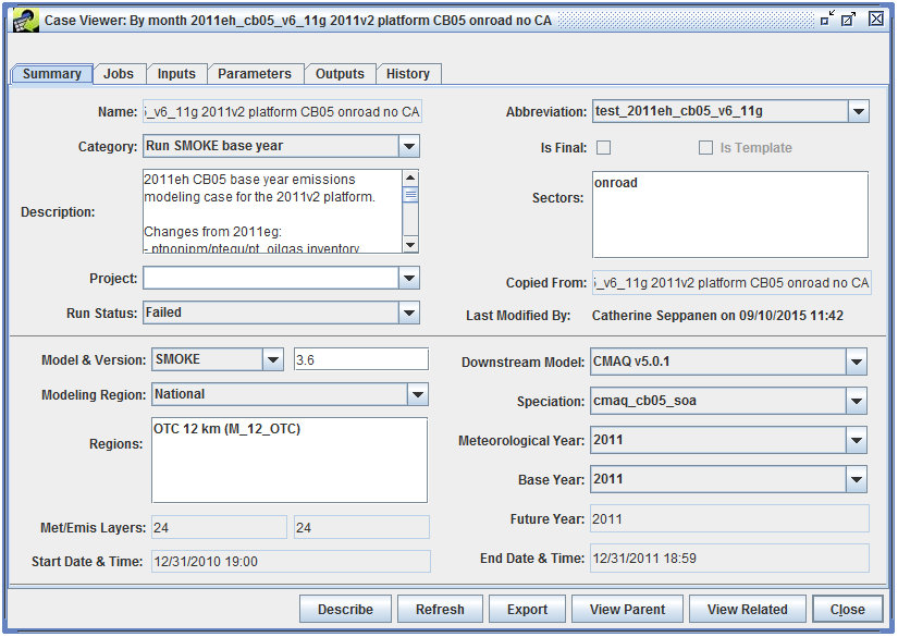
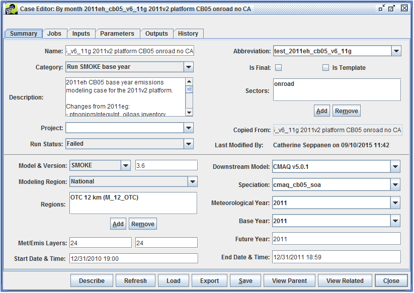
The Case Viewer and Case Editor windows split the case details into six tabs. Tbl. 5.3 gives a brief description of each tab.
| Tab | Description |
|---|---|
| Summary | Shows an overview of the case and high-level settings |
| Jobs | Work with the individual jobs that make up the case |
| Inputs | Select datasets that will be used as inputs to the case’s jobs |
| Parameters | Configure settings and other information needed to run the jobs |
| Outputs | View and export the output datasets created by the case’s jobs |
| History | View log and status messages generated by individual jobs |
There are several buttons that appear at the bottom of the Case Viewer and Case Editor windows. The actions for each button are described in Tbl. 5.4.
| Command | Description |
|---|---|
| Describe | Shows the case description in a larger window. If opened from the Case Editor window, the description can be edited (see Fig. 5.5). |
| Refresh | Reload the case details from the server. |
| Load (Case Editor only) | Manually load data created by CMAQ jobs into the EMF. |
| Export | Exports the case settings to text files. See Sec. 5.1.1. |
| Save (Case Editor only) | Save the current case. |
| View Parent | If the case was copied from another case, opens the Case Viewer showing the original case. |
| View Related | View other cases that either produce inputs used by the current case, or use outputs created by the current case. |
| Close | Closes the Case Viewer or Case Editor window |
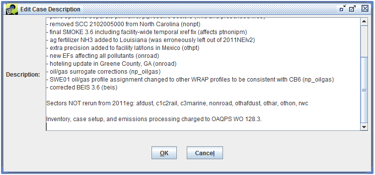
The Export button at the bottom of the Case Viewer or Case Editor window can be used to export the current case. Clicking the Export button will open the Export Case dialog shown in Fig. 5.6.
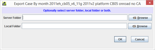
The case can be exported to text files either on the EMF server or directly to a local folder. After selecting the export location, click OK to export the case. The export process will create three text files, each named with the case’s name and abbreviation. Tbl. 5.5 describes the contents of the three files.
| File Name | Description |
|---|---|
| case_name_abbrev_Summary_Parameters.csv | Settings from the Summary tab, and a list of parameters for the case |
| case_name_abbrev_Jobs.csv | List of jobs for the case with settings for each job |
| case_name_abbrev_Inputs.csv | List of inputs for the case including the dataset name associated with each input |
The exported case data can be loaded back into the EMF using the Import button in the Case Manager window.
Fig. 5.7 shows the Summary tab in the Case Editor window.
The Summary tab shows a high-level overview of the case including the case’s name, abbreviation, and assigned category. Many of the fields on the Summary tab are listed in the Case Manager window as described in Tbl. 5.1.
The Is Final checkbox indicates that the case should be considered final and should not have any changes made to it. The Is Template checkbox indicates that the case is meant as a template for additional cases and should not be run directly. The EMF does not enforce any restrictions on cases marked as final or templates.
The Description textbox allows a detailed description of the case to be entered. The Describe button at the bottom of the Case Editor window will open the case description in a larger window for easier editing.
The Sectors box lists the sectors that have been associated with the case. Click the Add or Remove buttons to add or remove sectors from the list.
A case can optionally be assigned to a project using the Project pull-down menu.
If the case was copied from a different case, the parent case name will be listed by the Copied From label. This value is not editable. Clicking the View Parent button will open the copied from case.
The overall status of the case can be set using the Run Status pull-down menu. Available statuses are Not Started, Running, Failed, and Complete.
The Last Modified By field shows who last modified the case and when. This field is not editable.
The lower section of the Summary tab has various fields to set technical details about the case such as which model will be run, the downstream model (i.e. which model will be using the output from the case), and the speciation mechanism in use. These values will be available to the scripts that are run for each case job; see Sec. 5.2 for more information.
For the case shown in Fig. 5.7, the Start Date & Time is January 1, 2011 00:00 GMT and the End Date & Time is December 31, 2011 23:59 GMT. The EMF client has automatically converted these values from GMT to the local time zone of the client which is Eastern Daylight Time (GMT-5). Thus the values shown in the screenshot are correct, but confusing.
Fig. 5.8 shows the Jobs tab in the Case Editor window.
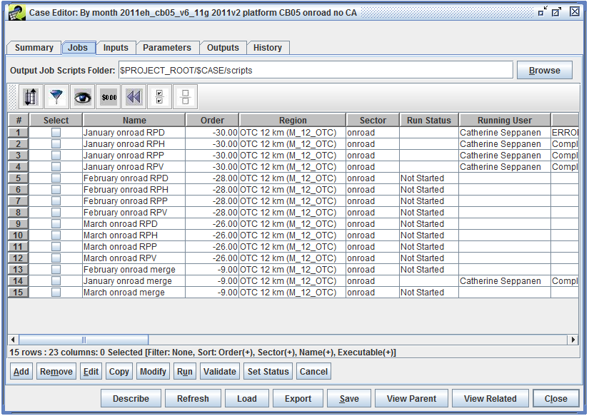
At the top of the Jobs tab is the Output Job Scripts Folder. When a job is run, the EMF creates a shell script in this folder. See Sec. 5.2 for more information about the script that the EMF writes and executes. Click the Browse button to set the scripts folder location on the EMF server. Otherwise, the folder location can be typed in the text field.
As shown in Fig. 5.8, the Output Job Scripts Folder can use variables to refer to case settings or parameters. In this case, the folder location is set to $PROJECT_ROOT/$CASE/scripts. PROJECT_ROOT is a case parameter defined in the Parameters tab with the value /data/em_v6.2/2011platform. The CASE variable refers to the case’s abbreviation: test_2011eh_cb05_v6_11g. Thus, the scripts for the jobs in the case will be written to the folder /data/em_v6.2/2011platform/test_2011eh_cb05_v6_11g/scripts.
To view the details of a particular job, select the job, then click the Edit button to bring up the Edit Case Job window (Fig. 5.9).
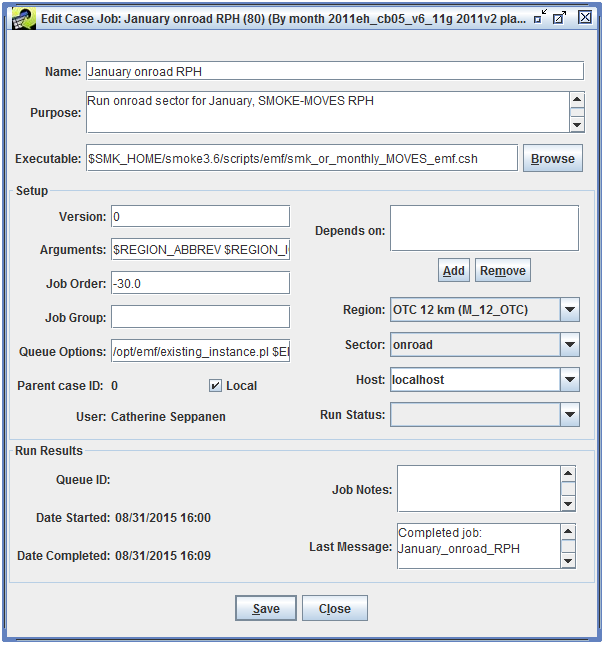
Tbl. 5.6 describes each field in the Edit Case Job window.
| Name | Description |
|---|---|
| Name | The name of the job. When setting up a job, the combination of the job’s name, region, and sector must be unique. |
| Purpose | A short description of the job’s purpose or functionality. |
| Executable | The script or program the job will run. |
| Setup | |
| Version | Can be used to mark the version of a particular job. |
| Arguments | A string of arguments to pass to the executable when the job is run. |
| Job Order | The position of this job in the list of jobs. |
| Job Group | Can be used to label related jobs. |
| Queue Options | Any commands that are needed when submitting the job to run (i.e. queueing system options, or a wrapper script to call). |
| Parent case ID | If this job was copied from a different case, shows the parent case’s ID. |
| Local | Can be used to indicate to other users if the job runs locally vs. remotely. |
| Depends on | TBA |
| Region | Indicates the region associated with the job. |
| Sector | Indicates the sector associated with the job. |
| Host | If set to anything other than localhost, the job is executed via SSH on the remote host. |
| Run Status | Shows the run status of the job. |
| Run Results | |
| Queue ID | Shows the queueing system ID, if the job is run on a system that provides this information. |
| Date Started | The date and time the job was last started. |
| Date Completed | The date and time the job completed. |
| Job Notes | User editable notes about the job run. |
| Last Message | The most recent message received while running the job. |
After making any edits to the job, click the Save button to save the changes. The Close button closes the Edit Case Job window.
To create a new job, click the Add button to open the Add a Job window as shown in Fig. 5.10.
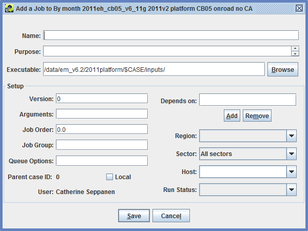
The Add a Job window has the same fields as the Edit Case Job window except that the Run Results section is not shown. See Tbl. 5.6 for more information about each input field. Once the job information is complete, click the Save button to save the new job. Click Cancel to close the Add a Job window without saving the new job.
An existing job can be copied to a different case or the same case using the Copy button. Fig. 5.11 shows the window that opens when copying a job.
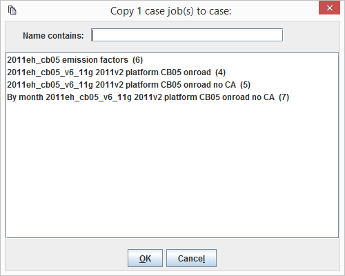
If multiple jobs need to be edited with the same changes, the Modify button can be used. This action opens the window shown in Fig. 5.12.
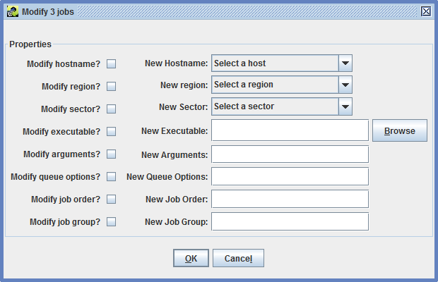
In the Modify Jobs window, check the checkbox next to each property to be modified. Enter the new value for the property. After clicking OK, the new value will be set for all selected jobs.
In the Jobs tab of the Case Editor window, the Validate button can be used to check the inputs for a selected job. The validation process will check each input for the job and report if any inputs use a non-final version of their dataset, or if any datasets have later versions available. If no later versions are found, the validation message “No new versions exist for selected inputs.” is displayed.
When the Inputs tab is initially viewed, the list of inputs will be empty as seen in Fig. 5.13.
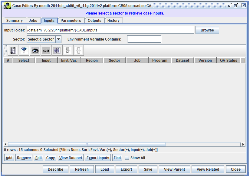
To view the inputs, use the Sector pull-down menu to select a sector associated with the case. In Fig. 5.14, the selected sector is All, so that all inputs for the case are displayed.
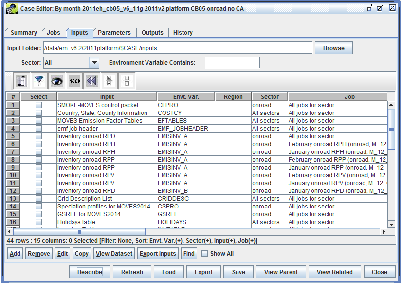
To view the details of an existing input, select the input, then click the Edit button to open the Edit Case Input window as shown in Fig. 5.15.
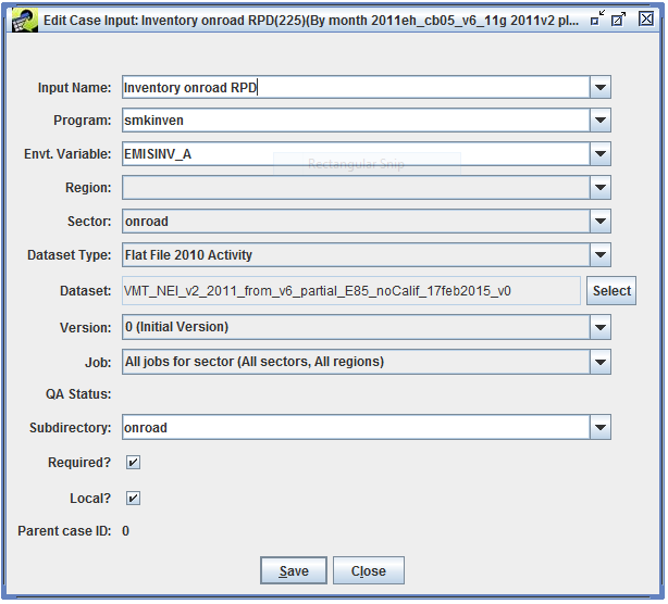
To create a new input, click the Add button to bring up the Add Input to Case window (Fig. 5.16).
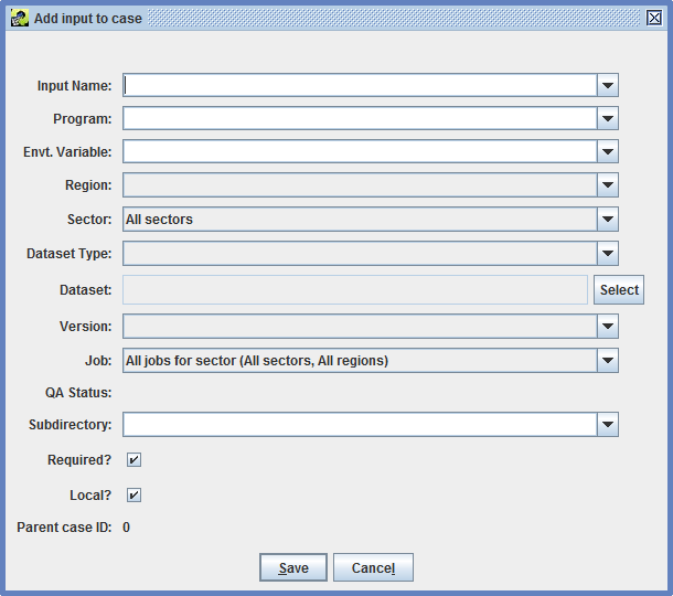
The Copy button can be used to copy an existing input to a different case. Fig. 5.17 shows the Copy Case Input window that opens when the Copy button is clicked.

To view the dataset associated with a particular input, click the View Dataset button to open the Dataset Properties View window for the selected input.
Like the Inputs tab, the Parameters tab will be empty when initially viewed, as shown in Fig. 5.18.
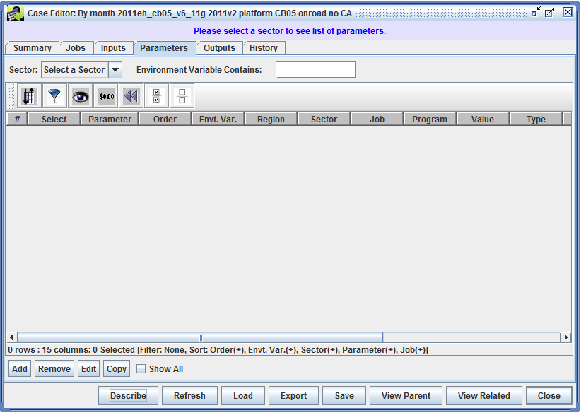
To view the parameters, use the Sector pull-down menu to select a sector. Fig. 5.19 shows the Parameters tab with the sector set to All, so that all parameters for the case are shown.
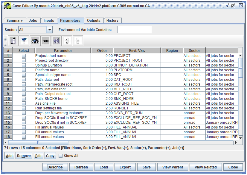
To view or edit the details of an existing parameter, select the parameter, then click the Edit button. This opens the parameter editing window as shown in Fig. 5.20.
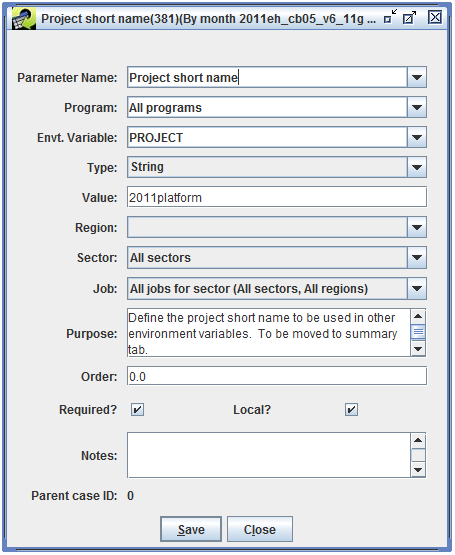
To create a new parameter, click the Add button and the Add Parameter to Case window will be displayed (Fig. 5.21).
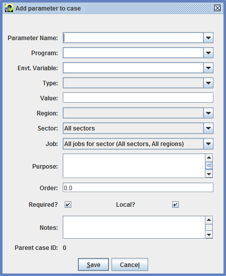
When initially viewed, the Outputs tab will be empty, as seen in Fig. 5.22.
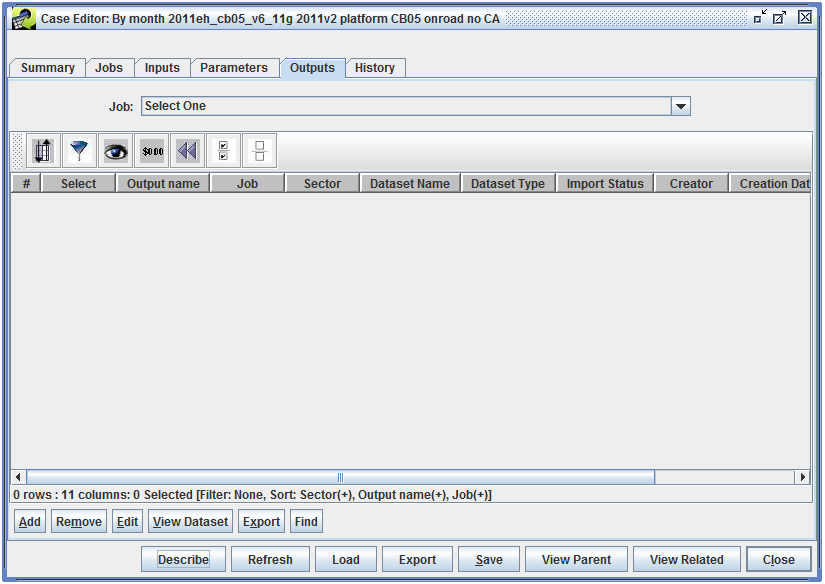
Use the Job pull-down menu to select a particular job and see the outputs for that job, or select “All (All sectors, All regions)” to view all the available outputs. Fig. 5.23 shows the Outputs tab with All selected.
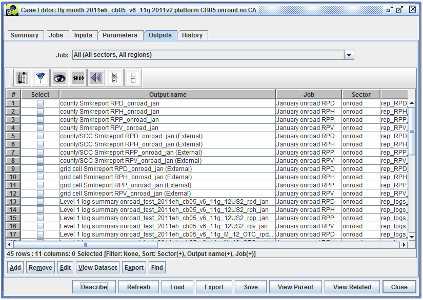
Tbl. 5.7 lists the columns in the table of case outputs. Most outputs are automatically registered when a case job is run, and the job script is responsible for setting the output name, dataset information, message, etc.
| Column | Description |
|---|---|
| Output Name | The name of the case output. |
| Job | The case job that created the output. |
| Sector | The sector associated with the job that created the output. |
| Dataset Name | The name of the dataset for the output. |
| Dataset Type | The dataset type associated with the output dataset. |
| Import Status | The status of the output dataset import. |
| Creator | The user who created the output. |
| Creation Date | The date and time when the output was created. |
| Exec Name | If set, indicates the executable that created the output. |
| Message | If set, a message about the output. |
Like the Outputs tab, the History tab is empty when initially viewed (Fig. 5.24).
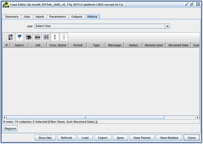
The history of a single job can be viewed by selecting that job from the Job pull-down menu, or the history of all jobs can be viewed by selecting “All (All sectors, All regions)”, as seen in Fig. 5.25.
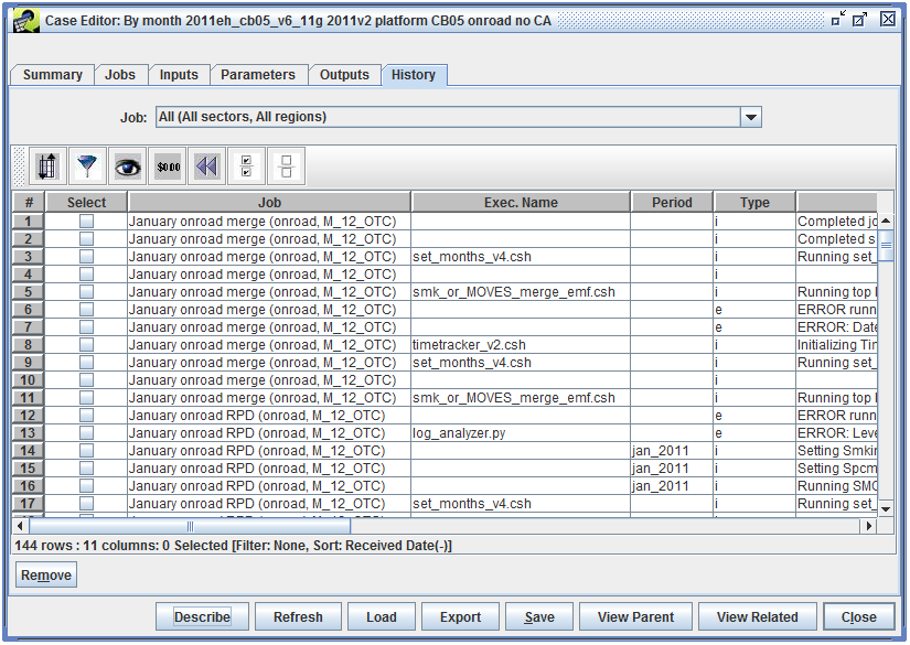
Messages in the History tab are automatically generated by the scripts that run for each case job. Each message will be associated with a particular job and the History tab will show when the message was received. Additionally, each message will have a type: i (info), e (error), or w (warning). The case job may report a specific executable and executable path associated with the message.
When a job is run, the EMF creates a shell script that will call the job’s executable. This script is created in the Output Job Scripts Folder specified in the Jobs tab of the Case Editor.
If the case includes an EMF_JOBHEADER input, the contents of this dataset are put at the beginning of the shell script. Next, all the environment variables associated with the job are exported in the script. Finally, the script calls the job’s executable with any arguments and queue options specified in the job.
In addition to the environment variables associated with a job’s inputs and parameters, Tbl. 5.8 and Tbl. 5.9 list the case and job settings that are automatically added to the script written by the EMF.
| Case Setting | Env. Var. | Example |
|---|---|---|
| abbreviation | $CASE | test_2011eh_cb05_v6_11g |
| base year | $BASE_YEAR | 2011 |
| future year | $FUTURE_YEAR | 2011 |
| model name and version | $MODEL_LABEL | SMOKE3.6 |
| downstream model | $EMF_AQM | CMAQ v5.0.1 |
| speciation | $EMF_SPC | cmaq_cb05_soa |
| start date & time | $EPI_STDATE_TIME | 2011-01-01 00:00:00.0 |
| end date & time | $EPI_ENDATE_TIME | 2011-12-31 23:59:00.0 |
| parent case | $PARENT_CASE | 2011eh_cb05_v6_11g_onroad_no_ca |
| Job Setting | Env. Var. | Example |
|---|---|---|
| sector | $SECTOR | onroad |
| job group | $JOB_GROUP | |
| region | $REGION | OTC 12 km |
| region abbreviation | $REGION_ABBREV | M_12_OTC |
| region gridname | $REGION_IOAPI_GRIDNAME | M_12_OTC |
The temporal allocation module in the Emissions Modeling Framework allows you to estimate inventory emissions for different time periods and resolutions. The module supports input inventories with annual totals, monthly totals, monthly average-day emissions, or daily totals. Using temporal allocation factors, the module can estimate monthly totals, monthly average-day values, daily totals, episodic totals, or episodic average-day values.
Under the main Manage menu, select Temporal Allocation to open the Temporal Allocation Manager. The Temporal Allocation Manager window will list existing temporal allocations as shown in Fig. 6.1.
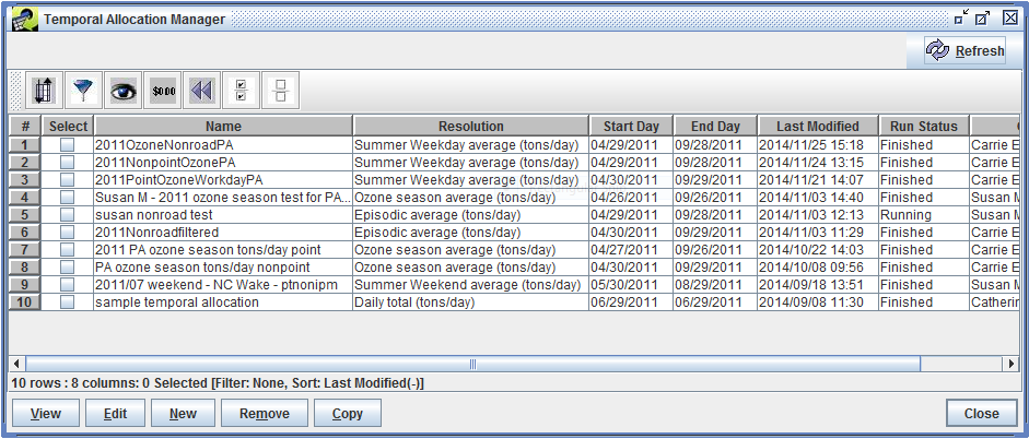
From the Temporal Allocation Manager, click the New button. The Edit Temporal Allocation window will open with the Summary tab selected (Fig. 6.2).
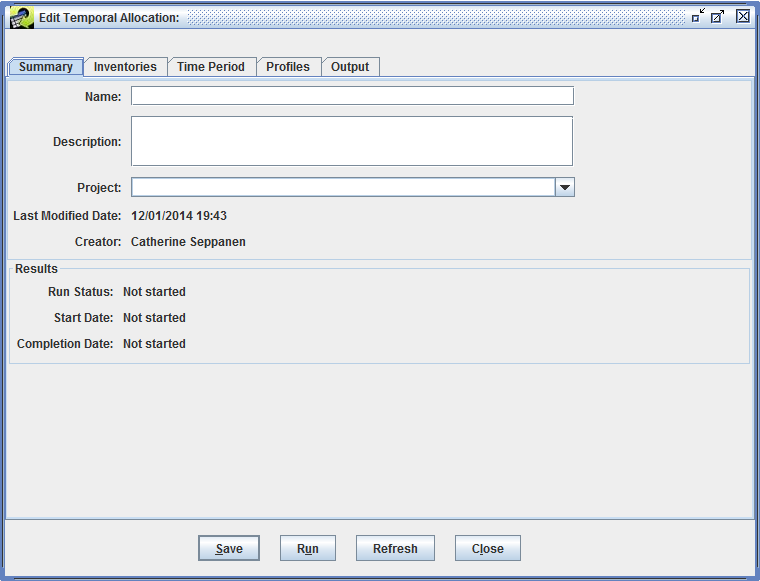
In the Edit Temporal Allocation window, the four tabs labeled Summary, Inventories, Time Period, and Profiles are used to enter the temporal allocation inputs. This information can be entered in any order; this guide goes through the tabs in order.
On the Summary tab, enter a unique name for the temporal allocation. You can optionally enter a description and select a project. The EMF will automatically set the last modified date and creator. Fig. 6.3 shows the Summary tab with details of the new temporal allocation entered.
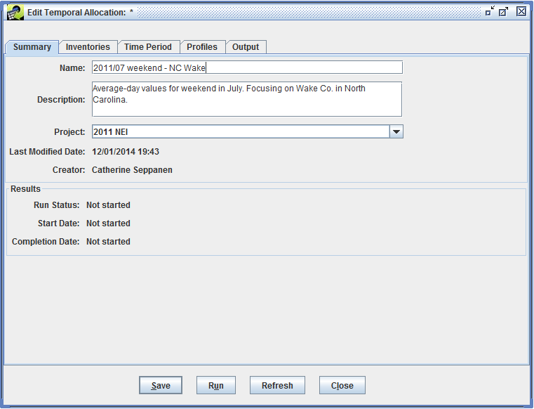
You can click the Save button from any tab in the Edit Temporal Allocation window to save the information you have entered. If you don’t enter a unique name, an error message will be displayed at the top of the window as shown in Fig. 6.4.
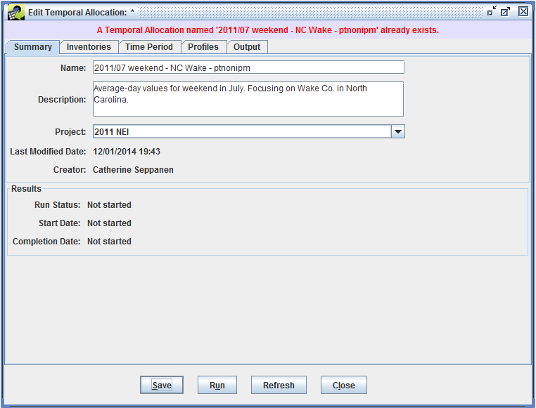
If you enter or update information and then try to close the edit window without saving, you will be asked if you would like to discard your changes. The prompt is shown in Fig. 6.5.
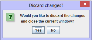
When your temporal allocation is successfully saved, a confirmation message is displayed at the top of the window.
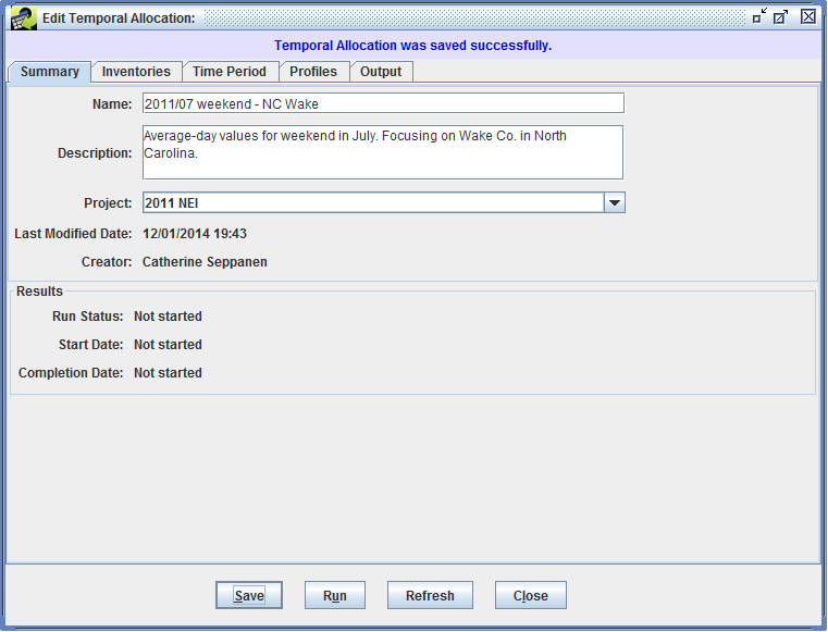
The Inventory tab of the Edit Temporal Allocation lists the inventories that will be processed by the temporal allocation. For a new temporal allocation, the list is initially empty as shown in Fig. 6.7.
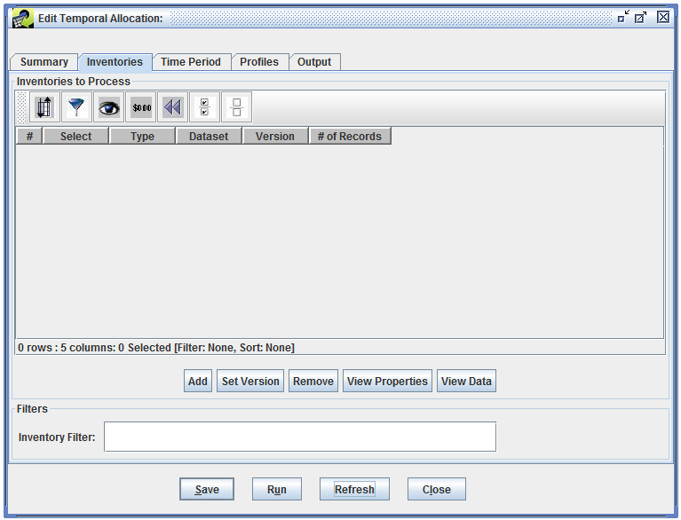
Click the Add button to select inventory datasets. A Select Datasets window will appear with the list of supported dataset types (Fig. 6.8).
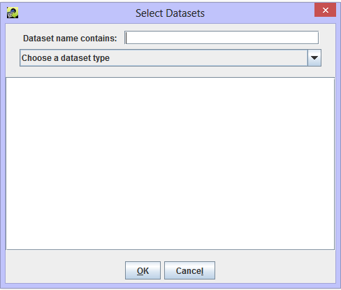
The temporal allocation module supports the following inventory dataset types:
Use the Choose a dataset type pull-down menu to select the dataset type you are interested in. A list of matching datasets will be displayed in the window as shown in Fig. 6.9.
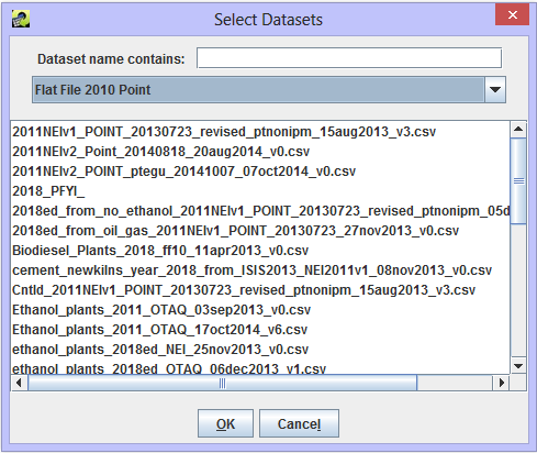
You can use the Dataset name contains field to filter the list of datasets as shown in Fig. 6.10.
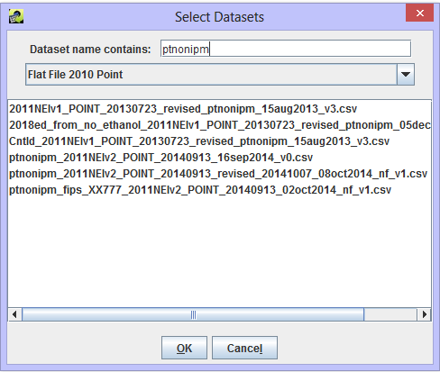
Click on the dataset names to select the datasets you want to add and then click the OK button. Fig. 6.11 shows the Select Datasets window with one dataset selected.
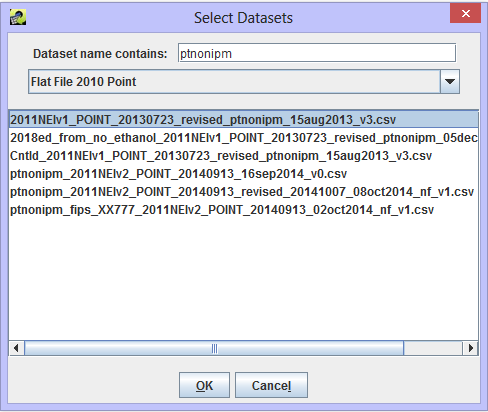
Your selected datasets will be displayed in the Inventories tab of the Edit Temporal Allocation window (Fig. 6.12).
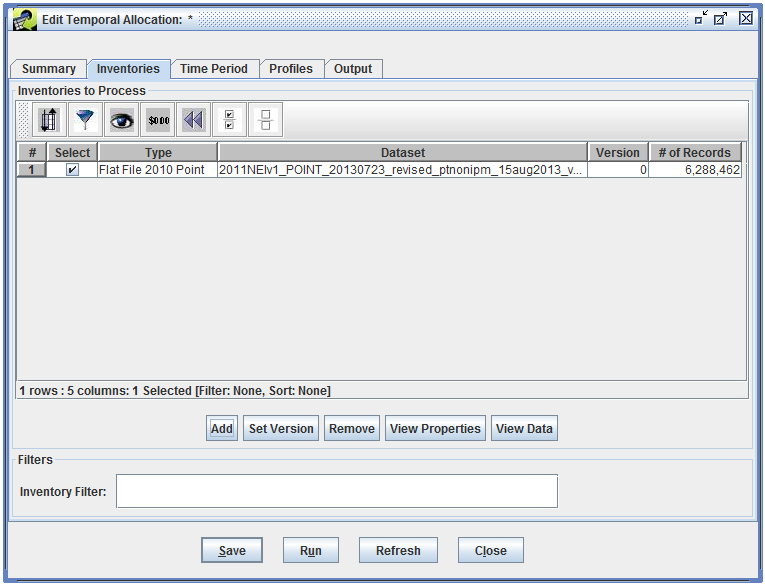
The module will automatically use the default version of each dataset. To change the dataset version, check the box next to the inventory and then click the Set Version button. A Set Version dialog will be displayed for each selected inventory as shown in Fig. 6.13.
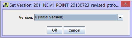
To remove an inventory dataset, check the box next to the dataset and then click the Remove button. The View Properties button will open the Dataset Properties View Sec. 3.5 for each selected dataset and the View Data button opens the Data Viewer (Fig. 3.21).
The Inventories tab also allows you to specify an inventory filter to apply to the input inventories. This is a general filter mechanism to reduce the total number of sources to be processed in the temporal allocation run. Fig. 6.14 shows an inventory filter that will match sources in Wake County, North Carolina and only consider CO emissions from the inventory.
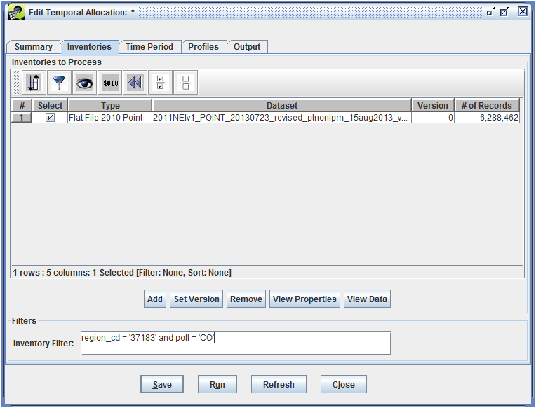
The temporal allocation module can process annual and monthly data from ORL and FF10 datasets. To determine if a given ORL inventory contains annual totals or monthly average-day values, the temporal allocation module first looks at the time period stored for the inventory dataset. (These dates are set using the Dataset Properties Editor [see Sec. 3.5] and are shown in the Time Period Start and Time Period End fields on the Summary tab.) If the dataset’s start and end dates are within the same month, then the inventory is treated as monthly data.
As a fallback from using the dataset time period settings, the module also looks at the dataset’s name. If the dataset name contains the month name or abbreviation like “_january” or “_jan”, then the dataset is treated as monthly data.
For FF10 inventories, the temporal allocation module will check if the inventory dataset contains any values in the monthly data columns (i.e. jan_value, feb_value, etc.). If any data is found, then the dataset is treated as monthly data.
The Time Period tab of the Edit Temporal Allocation window is used to set the desired output resolution and time period. Fig. 6.15 shows the Time Period tab for the new temporal allocation.
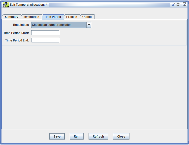
The temporal allocation module supports the following resolutions:
To set the time period for the temporal allocation, enter the start and end dates in the fields labeled Time Period Start and Time Period End. The dates should be formatted as MM/DD/YYYY. For example, to set the time period as May 1, 2008 thorugh October 31, 2008, enter “05/01/2008” in the Time Period Start text field and enter “10/31/2008” in the Time Period End text field. For monthly output, only the year and month of the time period dates will be used.
In Fig. 6.16, the output resolution has been set to Episodic weekend average and the time period is June 1, 2011 through August 31, 2011.
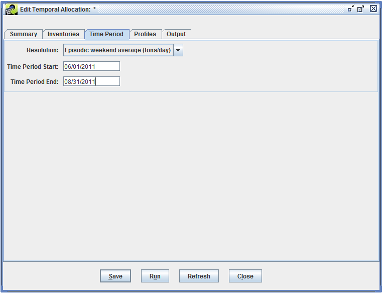
The Profiles tab of the Edit Temporal Allocation window is used to select the temporal cross-reference dataset and various profile datasets. The cross-reference dataset is used to assign temporal allocation profiles to each source in the inventory. A profile dataset contains factors to estimate emissions for different temporal resolutions. For example, a year-to-month profile will have 12 factors, one for each month of the year.
When editing a new temporal allocation, no datasets are selected initially as shown in Fig. 6.17.
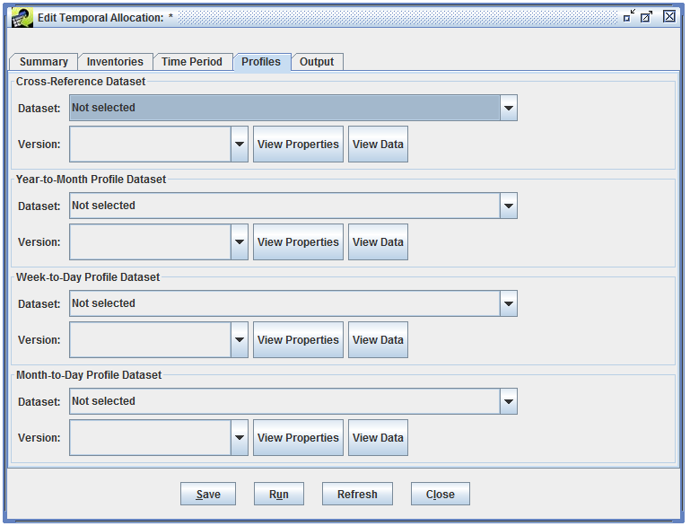
The Cross-Reference Dataset pull-down menu is automatically populated with datasets of type “Temporal Cross Reference (CSV)”. The format of this dataset is described in Sec. 6.4.
For annual input, year-to-month profiles are needed. The Year-To-Month Profile Dataset pull-down menu lists datasets of type “Temporal Profile Monthly (CSV)”.
For daily or episodic output, the inventory data will need estimates of daily data. The temporal allocation module supports using week-to-day profiles or month-to-day profiles. The Week-To-Day Profile Dataset pull-down menu lists available datasets of type “Temporal Profile Weekly (CSV)”. The Month-to-Day Profile Dataset pull-down shows datasets of type “Temporal Profile Daily (CSV)”.
The formats of the various profile datasets are described in Sec. 6.4.
Fig. 6.18 shows the Profiles tab with cross-reference, year-to-month profile, and week-to-day profile datasets selected.
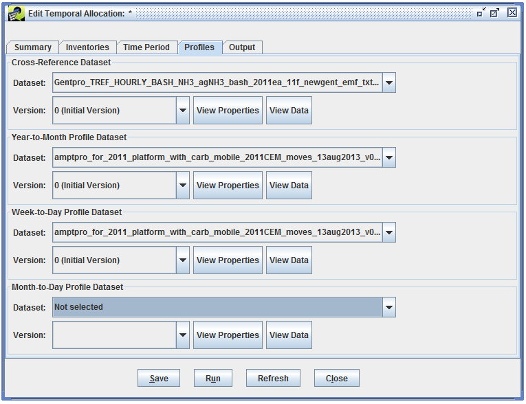
For each dataset, the default version will be selected automatically. The Version pull-down menu lists available versions for each dataset if you want to use a non-default version.
The View Properties button will open the Dataset Properties View (Sec. 3.5) for the associated dataset. The View Data button opens the Data Viewer (Fig. 3.21).
The Output tab will display the result datasets created when you run a temporal allocation. For a new temporal allocation, this window is empty as shown in Fig. 6.19.
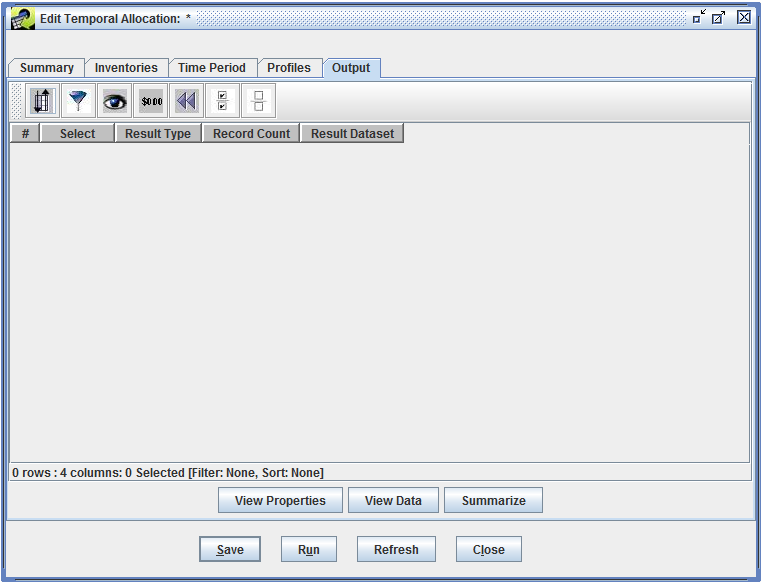
All temporal allocation runs are started from the Edit Temporal Allocation window. To run a temporal allocation, first open the Temporal Allocation Manager window from the main Manage menu. Check the box next to the temporal allocation you want to run and then click the Edit button.
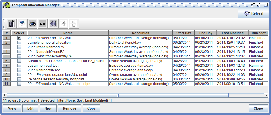
The Edit Temporal Allocation window will open for the temporal allocation you selected. Click the Run button at the bottom of the window to start running the temporal allocation.
If any problems are detected, an error message is displayed at the top of the Edit Temporal Allocation window (see Fig. 6.22 for an example). The following requirements must be met before a temporal allocation can be run:
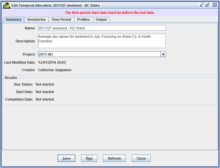
After starting the run, you’ll see a message at the top of the Edit Temporal Allocation window as shown in Fig. 6.23.
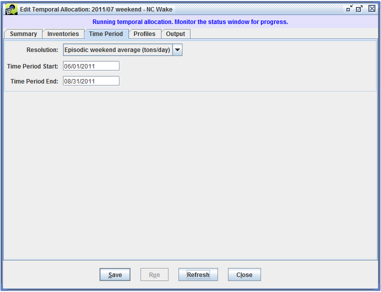
The EMF Status window (Sec. 2.6.5) will display updates as the temporal allocation is run. There are several steps in running a temporal allocation. First, any existing outputs for the temporal allocation are removed, indexes are created for the inventory datasets to speed up processing in the database, and the cross-reference dataset is cleaned to make sure the data is entered in a standard format.
Next, monthly totals and monthly average-day values are calculated from the input inventory data. The monthly values are stored in the monthly result output dataset which uses the “Temporal Allocation Monthly Result” dataset type. For annual input data, the year-to-month profiles are used to estimate monthly values. For monthly data from FF10 inventories, a monthly average-day value is calculated by dividing the monthly total value by the number of days in the month. For monthly data from ORL inventories, the monthly total is calculated by multiplying the monthly average-day value by the number of days in the month.
For daily and episodic output (i.e. the temporal allocation’s output resolution is not “Monthly average” or “Monthly total”), the next step is to calculate daily emissions. If a month-to-day profile is used, the monthly total value is multiplied by the appropriate factor from the month-to-day profile to calculate the emissions for each day.
Instead of month-to-day profiles, week-to-day profiles can be used. Week-to-day profiles contain 7 factors, one for each day of the week. To apply a weekly profile, the monthly average-day value is multiplied by 7 to get a weekly total value. Then, the weekly total is multiplied by the appropriate factor from the week-to-day profile to calculate the emissions for each day of the week. The calculated daily emission are stored in the daily result dataset which uses the dataset type “Temporal Allocation Daily Result”.
If the temporal allocation resolution is episodic totals or average-day, an episodic result dataset is created using the dataset type “Temporal Allocation Episodic Result”. This dataset will contain episodic totals and average-day values for the sources in the inventory. This values are calculated by summing the appropriate daily values and then dividing by the number of days to calculate the average-day values.
Once the temporal allocation has finished running, a status message “Finished Temporal Allocation run.” will be displayed. Fig. 6.24 shows the Status window after the temporal allocation has finished running.
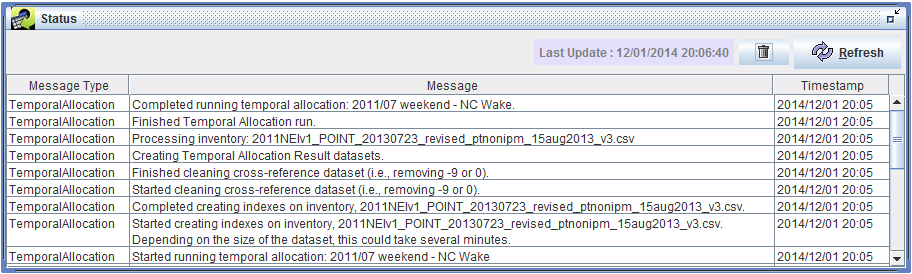
The Summary tab of the Edit Temporal Allocation window includes an overview of the run listing the status (Running, Finished, or Failed) and the start and completion date for the most recent run.
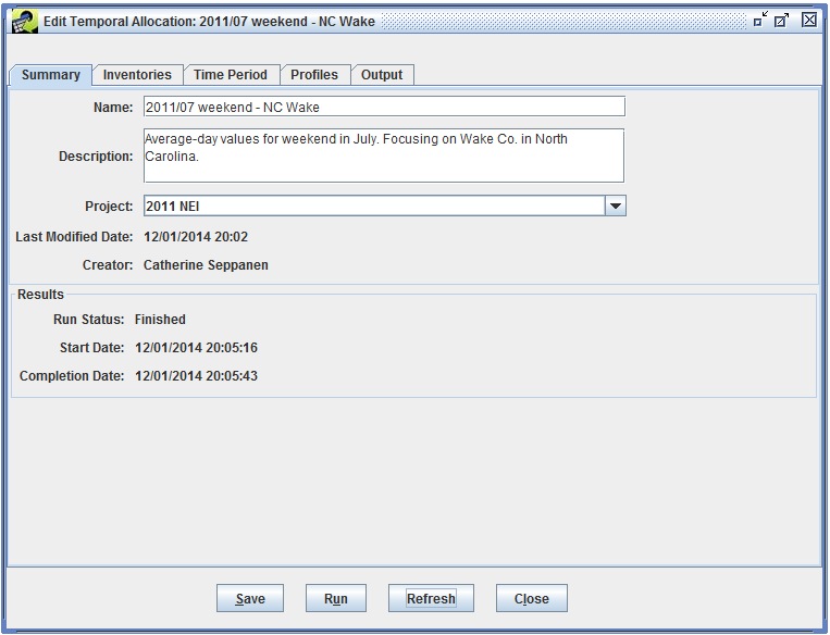
The Output tab of the Edit Temporal Allocation window will show the three result datasets from the run - monthly, daily, and episodic results.
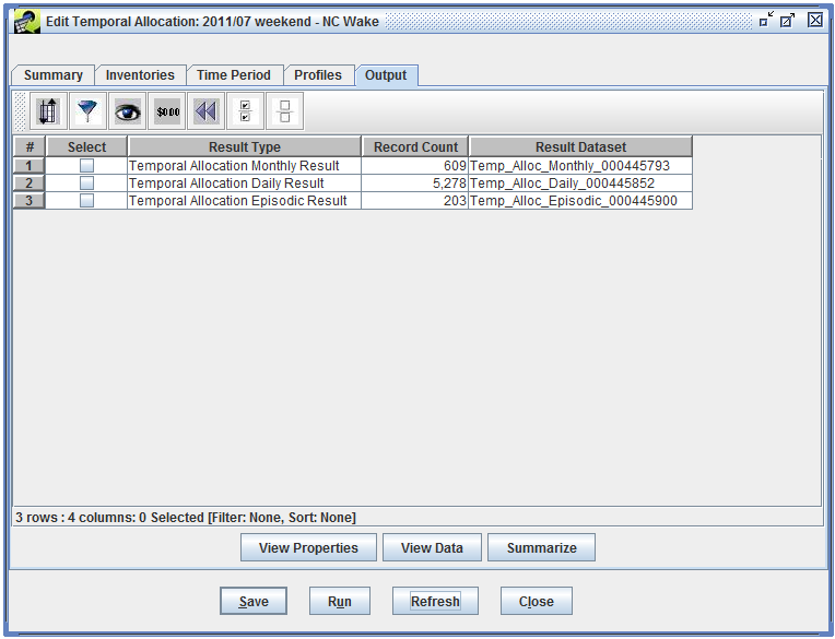
From the Output tab, you can select any of the result datasets and click the View Properties button to open the Dataset Properties View window (Sec. 3.5) for the selected dataset.
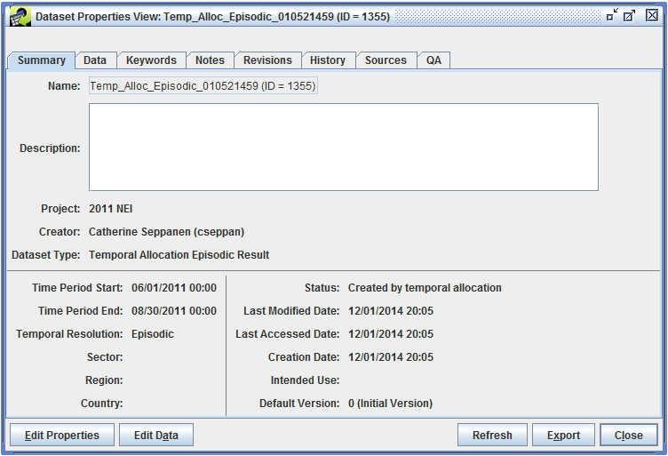
You can also access the result datasets from the Dataset Manager.
The View Data button will open the Data Viewer window (Fig. 3.21) for the selected dataset. Clicking the Summarize button will open the QA tab of the Dataset Properties Editor window (Sec. 3.5.8).
You can use QA steps to analyze the result datasets; see Sec. 4 for information on creating and running QA steps. The formats of the three types of result datasets are described in Sec. 6.5.
| Column | Name | Type | Description |
|---|---|---|---|
| 1 | SCC | VARCHAR(20) | Source Category Code (optional; enter zero for entry that is not SCC-specific) |
| 2 | FIPS | VARCHAR(12) | Country/state/county code (optional) |
| 3 | PLANTID | VARCHAR(20) | Plant ID/facility ID (optional - applies to point sources only; leave blank for entry that is not facility-specific) |
| 4 | POINTID | VARCHAR(20) | Point ID/unit ID (optional - applies to point sources only) |
| 5 | STACKID | VARCHAR(20) | Stack ID/release point ID (optional - applies to point sources only) |
| 6 | PROCESSID | VARCHAR(20) | Segment/process ID (optional - applies to point sources only) |
| 7 | POLL | VARCHAR(20) | Pollutant name (optional; enter zero for entry that is not pollutant-specific) |
| 8 | PROFILE_TYPE | VARCHAR(10) | Code indicating which type of profile this entry is for. Values used by the EMF are ‘MONTHLY’, ‘WEEKLY’, or ‘DAILY’. The format also supports hourly indicators ‘MONDAY’, ‘TUESDAY’, … ‘SUNDAY’, ‘WEEKEND’, ‘WEEKDAY’, ‘ALLDAY’, and ‘HOURLY’. |
| 9 | PROFILE_ID | VARCHAR(15) | Temporal profile ID |
| 10 | COMMENT | TEXT | Comments (optional; must be double quoted) |
| Column | Name | Type | Description |
|---|---|---|---|
| 1 | PROFILE_ID | VARCHAR(15) | Monthly temporal profile ID |
| 2 | JANUARY | REAL | Temporal factor for January |
| 3 | FEBRUARY | REAL | Temporal factor for February |
| 4 | MARCH | REAL | Temporal factor for March |
| … | … | … | … |
| 11 | OCTOBER | REAL | Temporal factor for October |
| 12 | NOVEMBER | REAL | Temporal factor for November |
| 13 | DECEMBER | REAL | Temporal factor for December |
| 14 | COMMENT | TEXT | Comments (optional; must be double quoted) |
| Column | Name | Type | Description |
|---|---|---|---|
| 1 | PROFILE_ID | VARCHAR(15) | Weekly temporal profile ID |
| 2 | MONDAY | REAL | Temporal factor for Monday |
| 3 | TUESDAY | REAL | Temporal factor for Tuesday |
| 4 | WEDNESDAY | REAL | Temporal factor for Wednesday |
| 5 | THURSDAY | REAL | Temporal factor for Thursday |
| 6 | FRIDAY | REAL | Temporal factor for Friday |
| 7 | SATURDAY | REAL | Temporal factor for Saturday |
| 8 | SUNDAY | REAL | Temporal factor for Sunday |
| 9 | COMMENT | TEXT | Comments (optional; must be double quoted) |
| Column | Name | Type | Description |
|---|---|---|---|
| 1 | PROFILE_ID | VARCHAR(15) | Daily temporal profile ID |
| 2 | MONTH | INTEGER | Calendar month |
| 3 | DAY1 | REAL | Temporal factor for day 1 of month |
| 4 | DAY2 | REAL | Temporal factor for day 2 of month |
| 5 | DAY3 | REAL | Temporal factor for day 3 of month |
| … | … | … | … |
| 31 | DAY29 | REAL | Temporal factor for day 29 of month |
| 32 | DAY30 | REAL | Temporal factor for day 30 of month |
| 33 | DAY31 | REAL | Temporal factor for day 31 of month |
| 34 | COMMENT | TEXT | Comments (optional; must be double quoted) |
The temporal allocation output datasets may contain sources from ORL or FF10 inventories. These two sets of inventory formats don’t use consistent names for the source characteristic columns. The temporal allocation formats use the ORL column names. Tbl. 6.1 shows how the column names map between FF10 and ORL inventories.
| FF10 Column Name | ORL Column Name | Description |
|---|---|---|
| REGION_CD | FIPS | State/county code, or state code |
| FACILITY_ID | PLANTID | Plant ID for point sources |
| UNIT_ID | POINTID | Point ID for point sources |
| REL_POINT_ID | STACKID | Stack ID for point sources |
| PROCESS_ID | SEGMENT | Segment for point sources |
| Column | Description |
|---|---|
| SCC | The source SCC from the inventory |
| FIPS | The source FIPS code from the inventory |
| PLANTID | For point sources, the plant ID/facility ID from the inventory |
| POINTID | For point sources, the point ID/unit ID from the inventory |
| STACKID | For point sources, the stack ID/release point ID from the inventory |
| PROCESSID | For point sources, the segment/process ID from the inventory |
| POLL | The source pollutant from the inventory |
| PROFILE_ID | The matched monthly temporal profile ID for the source; for monthly input data, this column will be blank |
| FRACTION | The temporal fraction applied to the source’s annual emissions for the current month; for monthly input data, the fraction will be 1 |
| MONTH | The calendar month for the current record |
| TOTAL_EMIS (tons/month) | The total emissions for the source and pollutant in the current month |
| DAYS_IN_MONTH | The number of days in the current month |
| AVG_DAY_EMIS (tons/day) | The average-day emissions for the source and pollutant in the current month |
| INV_RECORD_ID | The record number from the input inventory for this source |
| INV_DATASET_ID | The numeric ID of the input inventory dataset |
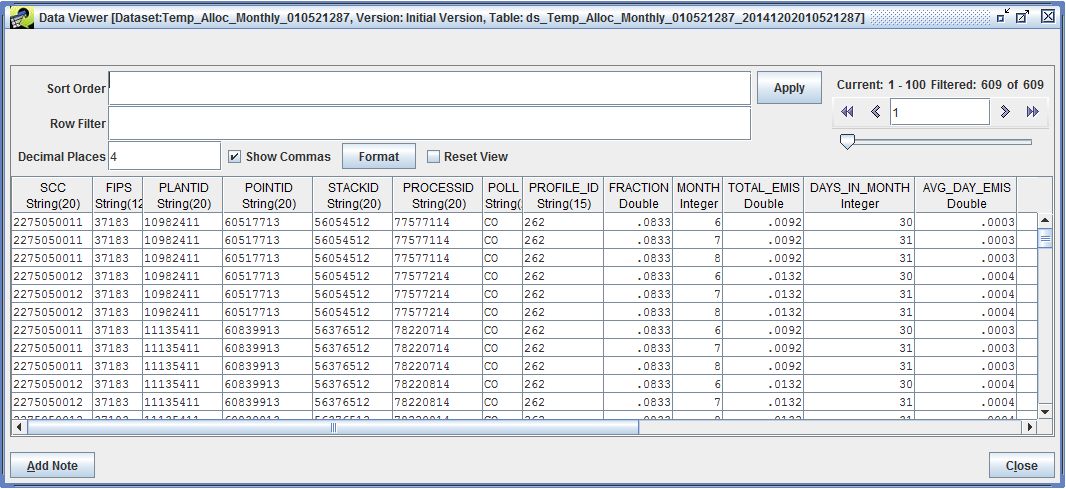
| Column | Description |
|---|---|
| SCC | The source SCC from the inventory |
| FIPS | The source FIPS code from the inventory |
| PLANTID | For point sources, the plant ID/facility ID from the inventory |
| POINTID | For point sources, the point ID/unit ID from the inventory |
| STACKID | For point sources, the stack ID/release point ID from the inventory |
| PROCESSID | For point sources, the segment/process ID from the inventory |
| POLL | The source pollutant from the inventory |
| PROFILE_TYPE | The type of temporal profile used for the source; currently only the WEEKLY type is supported |
| PROFILE_ID | The matched temporal profile ID for the source |
| FRACTION | The temporal fraction applied to the source’s monthly emissions for the current day |
| DAY | The date for the current record |
| TOTAL_EMIS (tons/day) | The total emissions for the source and pollutant for the current day |
| INV_RECORD_ID | The record number from the input inventory for this source |
| INV_DATASET_ID | The numeric ID of the input inventory dataset |
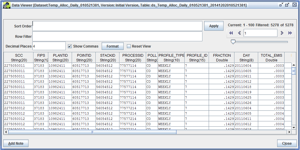
| Column | Description |
|---|---|
| SCC | The source SCC from the inventory |
| FIPS | The source FIPS code from the inventory |
| PLANTID | For point sources, the plant ID/facility ID from the inventory |
| POINTID | For point sources, the point ID/unit ID from the inventory |
| STACKID | For point sources, the stack ID/release point ID from the inventory |
| PROCESSID | For point sources, the segment/process ID from the inventory |
| POLL | The source pollutant from the inventory |
| TOTAL_EMIS (tons) | The total emissions for the source and pollutant in the episode |
| DAYS_IN_EPISODE | The number of days in the episode |
| AVG_DAY_EMIS (tons/day) | The average-day emissions for the source and pollutant in the episode |
| INV_RECORD_ID | The record number from the input inventory for this source |
| INV_DATASET_ID | The numeric ID of the input inventory dataset |
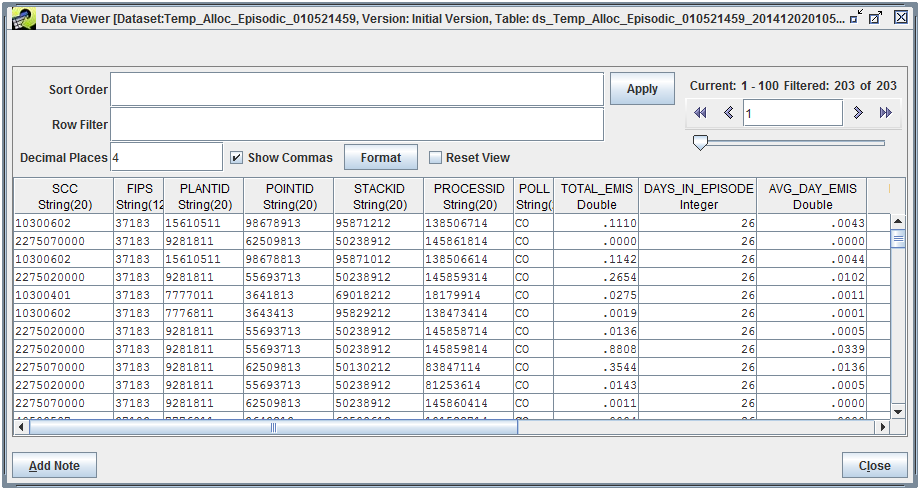
| Column | Description |
|---|---|
| SCC | The source SCC from the inventory |
| FIPS | The source FIPS code from the inventory |
| PLANTID | For point sources, the plant ID/facility ID from the inventory |
| POINTID | For point sources, the point ID/unit ID from the inventory |
| STACKID | For point sources, the stack ID/release point ID from the inventory |
| PROCESSID | For point sources, the segment/process ID from the inventory |
| POLL | The source pollutant from the inventory |
| PROFILE_ID | The matched temporal profile ID for the source |
| MESSAGE | Message describing the issue with the source |
The inventory projection process involves taking a base year inventory and projecting it to a future year inventory based on expected future activity levels and emissions controls. Within the EMF, inventory projection is accomplished using the “Project Future Year Inventory” (PFYI) strategy in the Control Strategy Tool (CoST) module. The Project Future Year Inventory control strategy matches a set of user-defined Control Programs to selected emissions inventories to estimate the emissions reductions in the target future year specified by the user. The output of the PFYI strategy can be used to generate a future year emissions inventory.
Control programs are used to describe the expected changes to the base year inventory in the future. The data includes facility/plant closure information, control measures and their associated emissions impacts, growth or reduction factors to account for changes in activity levels, and other adjustments to emissions such as caps or replacements.
The CoST module is primarily used to estimate emissions reductions and costs incurred by applying different sets of control measures to emissions sources in a given year. CoST allows users to choose from several different algorithms (Control Strategies) for matching control measures to emission sources. Control strategies include “Maximum Emissions Reduction” (what is the maximum emissions reduction possible regardless of cost?) and “Least Cost” (what combination of control measures achieves a targeted emissions reduction at the least cost?).
Inventory projection has some underlying similarities to the “what if” control scenario processing available in CoST. For example, projecting an inventory requires a similar inventory source matching process and applying various factors to base emissions. However, there are some important differences between the two types of processing:
| “What if” control strategies | Inventory projection |
|---|---|
| Estimates emissions reductions and costs for the same year as the input inventory | Estimates emissions changes for the selected future year |
| More concerned with cost estimates incurred by applying different control measures | Minimal support for cost estimates; primary focus is emissions changes |
| Matches sources with control measures from the Control Measure Database (CMDB) | Matches sources to data contained in user-created Control Programs |
This section will detail the “Project Future Year Inventory” control strategy available in CoST. More information on general use of CoST is available in the CoST User’s Guide.
Fig. 7.1 shows the various datasets and processing steps used for inventory projection within the EMF.
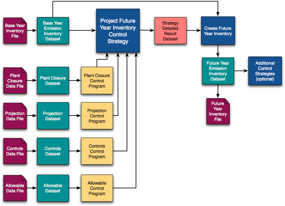
One or more base year inventories are imported into the EMF as inventory datasets. Files containing the control program data such as plant closures, growth or reduction factors (projection data), controls, and caps and replacements (allowable data) are also imported as datasets.
For each growth or control dataset, the user creates a Control Program. A Control Program specifies the type of program (i.e. plant closures, control measures to apply, growth or reduction factors) and the start and end date of the program. The dataset associated with the program identifies the inventory sources affected by the program and the factors to apply (e.g. the control efficiency of the associated control measure or the expected emissions reduction in the future year).
To create a Project Future Year Inventory control strategy, the user selects the input base year inventories and control programs to consider. The primary output of the control strategy is a Strategy Detailed Result dataset for each input inventory. The Strategy Detailed Result dataset consists of pairings of emission sources and control programs, each of which contains information about the emission adjustment that would be achieved if the control program were to be applied to the source.
The Strategy Detailed Result dataset can optionally be combined with the input inventory to create a future year inventory dataset. This future year inventory dataset can be exported to an inventory data file. The future year inventory dataset can also be used as input for additional control strategies to generate controlled future year emissions.
The Project Future Year Inventory strategy uses various types of Control Programs to specify the expected changes to emissions between the base year and the future year. Each Control Program has a start date indicating when the control program takes effect, an optional end date, and an associated dataset which contains the program-specific factors to apply and source-matching information. There are four major types of control programs: Plant Closure, Projection, Control, and Allowable.
A Plant Closure Control Program identifies specific plants to close. Each record in the plant closure dataset consists of:
Using the source matching options, you can specify particular stacks to close or close whole plants.
A Projection Control Program is used to apply growth or reduction factors to inventory emissions. Each record in the projection dataset consists of:
A Control-type Control Program is used to apply replacement or add-on control measures to inventory emissions. Each record in the control dataset consists of:
An Allowable Control Program is used to apply caps on inventory emissions or replacements to inventory emissions. Allowable Control Programs are applied after the other types of programs so that the impacts of the other programs can be accounted for when checking for emissions over the specified cap. Each record in the allowable dataset consists of:
Each Control Program is associated with a dataset. Tbl. 7.1 lists the EMF dataset types corresponding to each Control Program type. The Control Program datasets were designed to be compatible with the SMOKE GCNTL (growth and controls) input file which uses the term “packet” to refer to the different types of control program data; the same term is used in the EMF.
| Control Program Type | Dataset Types |
|---|---|
| Allowable | Allowable Packet, Allowable Packet Extended |
| Control | Control Packet, Control Packet Extended |
| Plant Closure | Plant Closure Packet (CSV), Facility Closure Extended |
| Projection | Projection Packet, Projection Packet Extended |
The dataset formats named with “Extended” add additional options beyond the SMOKE-based formats. These extended formats use the same source information fields as Flat File 2010 inventories and also support monthly factors in addition to annual values. Tbl. 7.2 shows how the column names map between the extended and non-extended dataset formats.
| Extended Format Column Name | Non-Extended Format Column Name | Description |
|---|---|---|
| REGION_CD | FIPS | State/county code, or state code |
| FACILITY_ID | PLANTID | Plant ID for point sources |
| UNIT_ID | POINTID | Point ID for point sources |
| REL_POINT_ID | STACKID | Stack ID for point sources |
| PROCESS_ID | SEGMENT | Segment for point sources |
| MACT | REG_CD | Maximum Achievable Control Technology (MACT) code |
The file formats for each control program dataset are listed in Sec. 7.7.
When building Control Program dataset records, you can use various combinations of source matching information depending on the level of specificity needed. For example, you could create a projection factor that applies to all sources with a particular SCC in the inventory regardless of geographic location. In this case, the SCC code would be specified but the region code would be left blank. If you need a different factor for particular regions, you can add additional records that specify both the SCC and region code with the more specific factor.
When matching the Control Program dataset records to inventory sources, more specific matches will be used over less specific ones. In the case of ties, a defined hierarchy is used to rank the matches. This hierarchy is listed in Sec. 7.8.
The main interface for creating and editing Control Programs is the Control Program Manager. To open the Control Program Manager, select Control Programs from the main Manage menu at the top of the EMF window. A list of existing control programs is displayed as shown in Fig. 7.2.
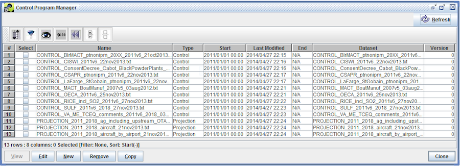
Tbl. 7.3 describes each column in the Control Program Manager window.
| Column | Description |
|---|---|
| Name | A unique name or label for the control program. |
| Type | The type of this control program. Options are Allowable, Control, Plant Closure, or Projection. |
| Start | The start date of the control program. Used when selecting control programs to apply in a strategy’s target year. |
| Last Modified | The most recent date and time when the control program was modified. |
| End | The end date of the control program. Used when selecting control programs to apply in a strategy’s target year. If not specified, N/A will be displayed. |
| Dataset | The name of the dataset associated with the control program. |
| Version | The version of the associated dataset that the control program will use. |
Using the Control Program Manager, you can select the control programs you want to work with by clicking the checkboxes in the Select column and then perform various actions related to those control programs. Tbl. 7.4 lists the buttons along the bottom of the Control Program Manager window and describes the action for each button.
| Command | Description |
|---|---|
| View | Not currently active. |
| Edit | Opens an Edit Control Program window for each of the selected control programs. |
| New | Opens a New Control Program window to create a new control program. |
| Remove | Deletes the selected control programs. Only the control program’s creator or an EMF administrator can delete a control program. |
| Copy | Creates a copy of each selected control program with a unique name. |
| Close | Closes the Control Program Manager window. |
From the Control Program Manager, click the New button at the bottom of the window. The window to create a new control program is displayed as shown in Fig. 7.3.
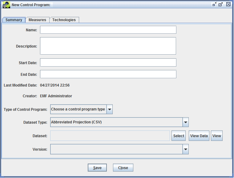
On the Summary tab, you can enter the details of the control program. Tbl. 7.5 describes each field.
| Field | Description |
|---|---|
| Name | Enter a unique name or label for this control program; required. |
| Description | Enter a description of the control program; optional. |
| Start Date | The start date for the control program formatted as MM/DD/YYYY; required. When running a Project Future Year Inventory strategy, only control programs whose start date falls within the strategy’s Target Year will be considered. |
| End Date | The end date for the control program formatted as MM/DD/YYYY; optional. If specified, the end date will be compared to the control strategy’s Target Year when deciding which control programs to consider. |
| Last Modified Date | Last modification date and time of the control program; automatically set by the EMF. |
| Creator | The EMF user who created the control program; automatically set by the EMF. |
| Type of Control Program | Select from the list of four control program types: Allowable, Control, Plant Closure, or Projection; required. |
| Dataset Type | Select the dataset type corresponding to the dataset you want to use for this control program. |
| Dataset | Click the Select button to open the dataset selection window as shown in Fig. 7.4. Only datasets matching the selected dataset type are displayed. Select the dataset you want to use for this Control Program and click the OK button. You can use the Dataset name contains search box to narrow down the list of datasets if needed. |
| Version | After you’ve selected the dataset, the Version pull-down lists the available versions of the dataset with the default version selected. You can select a different version of the dataset if appropriate. |
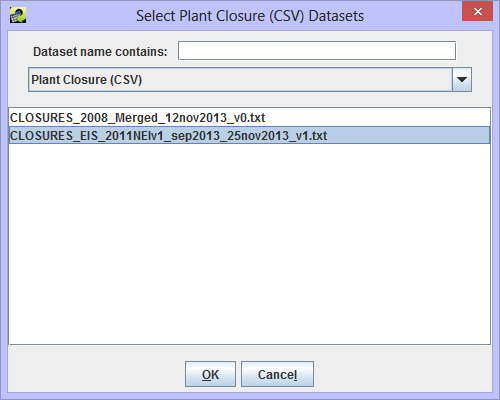
Fig. 7.5 shows the New Control Program window with the data fields filled out. Once you’ve finished entering the details of the new control program, click the Save button to save the control program.
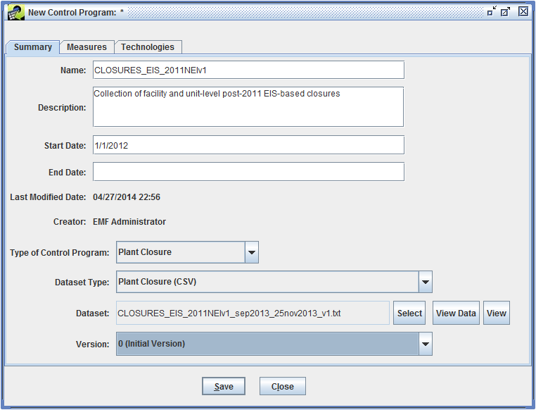
Once a dataset has been selected for a control program, the View Data and View buttons to the right of the dataset name will open the Data Viewer (Fig. 3.21) or Dataset Properties View (Sec. 3.5) for the selected dataset.
The Measures and Technologies tabs in the Edit Control Program window are only used when working with Control-type Control Programs.
When a Control-type control program is used in a Project Future Year Inventory control strategy, CoST will try to match each applied control packet record to a control measure in the Control Measure Database in order to estimate associated costs. You can specify a list of probable control measures or control technologies when you define the control program to limit the potential matches.
In the Edit Control Program window, the Measures tab (Fig. 7.6) lets you specify the control measures to include.
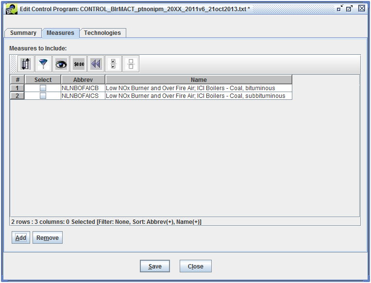
Click the Add button to open the Select Control Measures window. As shown in Fig. 7.7, the Select Control Measures window lists all the defined control measures including the control measure’s name, abbreviation, and major pollutant.
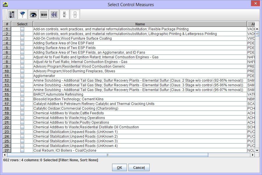
You can use the filtering and sorting options to find the control measures of interest. Select the control measures you want to add then click the OK button to add the control measures to the Control Program and return to the Edit Control Program window.
To remove control measures, select the appropriate control measures, then click the Remove button.
The Technologies tab in the Edit Control Program window (Fig. 7.8) allows you to specify particular control technologies associated with the control program.
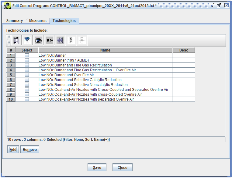
Click the Add button to open the Select Control Technologies window. As shown in Fig. 7.9, the Select Control Technologies window lists all the defined control technologies by name and description.
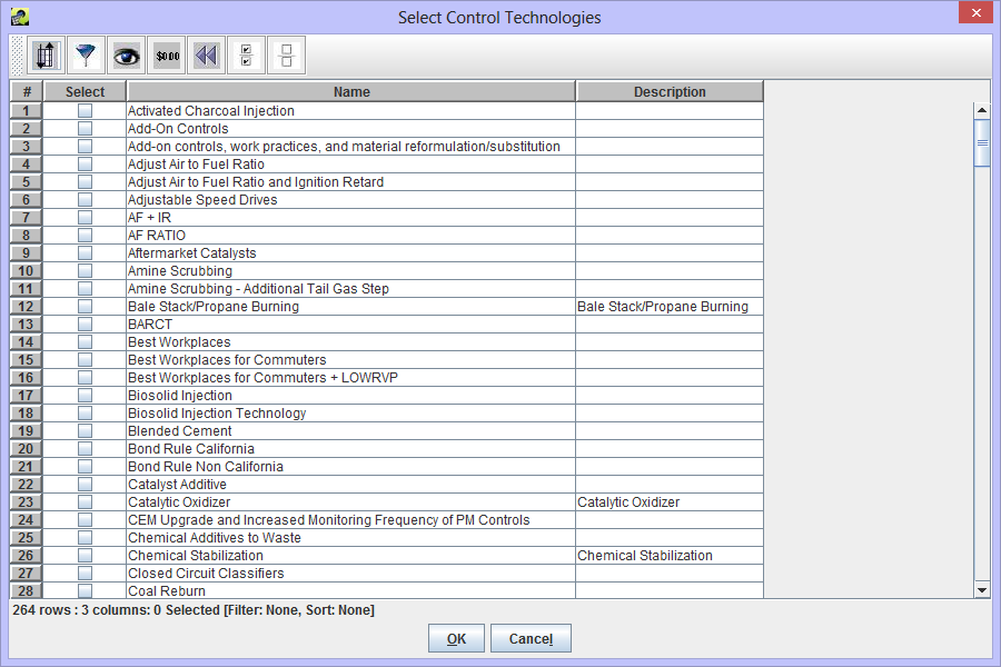
You can use the filtering and sorting options to find the control technologies of interest. Select the control technologies you want to add then click the OK button to add the control technologies to the Control Program and return to the Edit Control Program window.
To remove control technologies, select the appropriate control technologies, then click the Remove button.
To create a Project Future Year Inventory Control Strategy, first open the Control Strategy Manager by selecting Control Strategies from the main Manage menu. Fig. 7.10 shows the Control Strategy Manager window.
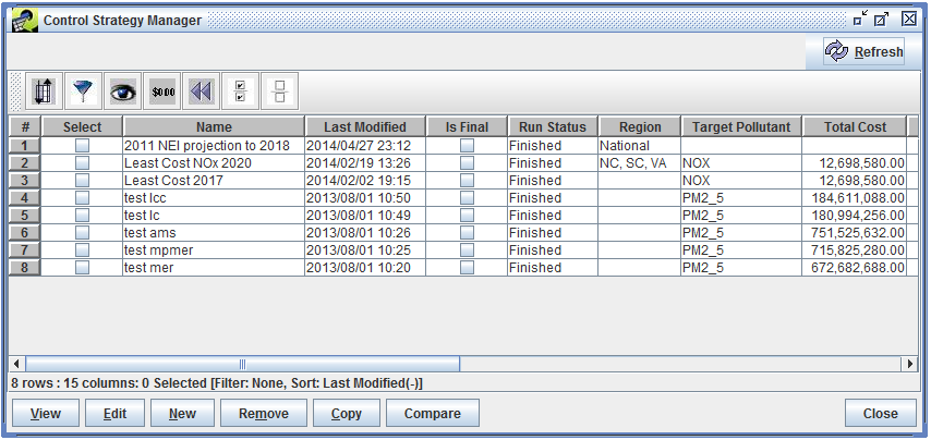
Click the New button to start creating the control strategy. You will first be prompted to enter a unique name for the control strategy as shown in Fig. 7.11.
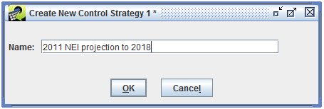
Almost all of the strategy parameters for the Project Future Year Inventory strategy have the same meaning and act in the same way as they do for the Maximum Emissions Reduction strategy, such as cost year, inventory filter, and county dataset. This section focuses on parameters or inputs that differ for the Project Future Year Inventory strategy type.
The Summary tab displays high-level parameters about the control strategy (Fig. 7.12).
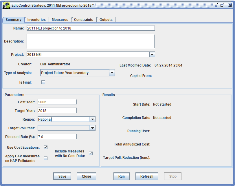
Parameters of interest for the Project Future Year Inventory strategy:
Type of Analysis: Project Future Year Inventory
Target Year: The target year represents the future year to which you are projecting the inventory. The target year is used when building the various cutoff dates (control compliance and plant closure effective dates) to evaluate whether or not certain control programs are applied to an inventory.
Target Pollutant: The target pollutant is not used for the Project Future Year Inventory control strategy.
The Project Future Year Inventory strategy can use inventories in the following dataset types: Flat File 2010 Point, Flat File 2010 Nonpoint, ORL point, ORL nonpoint, ORL nonroad, or ORL nonroad. Multiple inventories can be processed in a single strategy. Note that multiple versions of the inventories may be available, and the appropriate version of each inventory must be selected prior to running a control strategy.
The Programs tab in the Edit Control Strategy window is used to select which control programs should be considered in the strategy. Fig. 7.13 shows the Programs tab for an existing control strategy.
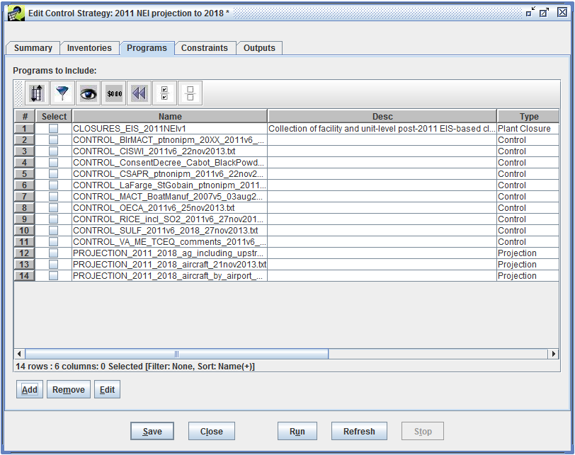
Click the Add button to bring up the Select Control Programs window as shown in Fig. 7.14.
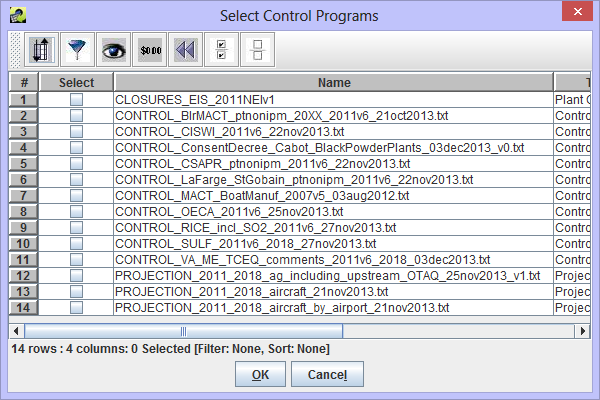
In the Select Control Programs window, you can select which control programs to use in your PFYI control strategy. The table displays the name, control program type, and description for all defined control programs. You can use the filter and sorting options to help find the control programs you are interested in. Select the checkbox next to each control program to add and then click the OK button to return to the Programs tab.
To remove control programs from the strategy, select the programs to remove and then click the Remove button. The Edit button will open an Edit Control Program window for each of the selected control programs.
More than one of the same type of control program can be added to a strategy. For example, you could add three Plant Closure Control Programs: Cement Plant Closures, Power Plant Closures, and Boiler Closures. All three of these control programs would be evaluated and a record of the evaluation would be stored in the Strategy Detailed Result. If there happen to be multiple Projection, Control, or Allowable Type Control Programs added to a strategy, packets of the same type are merged into one packet during the matching analysis so that no duplicate source-control-packet pairings are created. Duplicate records will be identified during the run process and the user will be prompted to remove duplicates before the core algorithm performs the projection process.
Fig. 7.15 shows the Constraints tab for a Project Future Year Inventory strategy. The only constraint used by PFYI strategies is a strategy-specific constraint named Minimum Percent Reduction Difference for Predicting Controls (%). This constraint determines whether a predicted control measure has a similar percent reduction to the percent reduction specified in the Control Program Control Packet.
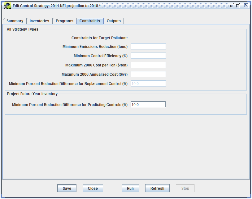
To run the Project Future Year Inventory control strategy, click the Run button at the bottom of the Edit Control Strategy window. The EMF will begin running the strategy. Check the Status window (Sec. 2.6.5) to monitor the status of the run.
The Project Future Year Inventory strategy processes Control Programs in the following order:
The Control analysis is dependent on the Projection analysis; likewise, the Allowable analysis is dependent on the Projection and Control analyses. The adjusted source emission values need to be carried along from each analysis step to make sure each portion of the analysis applies the correct adjustment factor. For example, a source could be projected, and also controlled, in addition to having a cap placed on the source. Or, a source could have a projection or control requirement, or perhaps just a cap or replacement requirement.
The main output for each control strategy is a table called the Strategy Detailed Result. This dataset consists of pairings of emission sources and control programs, each of which contains information about the emission adjustment that would be achieved if the control program were to be applied to the source, along with the cost of application. The Strategy Detailed Result table can be used with the original input inventory to produce, in an automated manner, a controlled emissions inventory that reflects implementation of the strategy; this inventory includes information about the control programs that have been applied to the controlled sources. The controlled inventory can then be directly input to the SMOKE modeling system to prepare air quality model-ready emissions data. In addition, comments are placed at the top of the inventory file to indicate the strategy that produced it and the settings of the high-level parameters that were used to run the strategy.
The columns in the Strategy Detailed Result dataset are described in Sec. 7.9, Tbl. 7.14.
In additional to the Strategy Detailed Result dataset, CoST automatically generates a Strategy Messages dataset. The Strategy Messages output provides useful information that is gathered while the strategy is running. This output can store ERROR and WARNING types of messages. If an ERROR is encountered during the prerun validation process, the strategy run will be canceled and the user can peruse this dataset to see what problems the strategy has (e.g., duplicate packet records).
The columns in the Strategy Messages dataset are described in Sec. 7.9, Tbl. 7.15.
After the Project Future Year Inventory control strategy has been run, you can create a future year emissions inventory. From the Outputs tab, select the Strategy Detailed Result for the base year inventory and select the Controlled Inventory radio button as shown in Fig. 7.16.
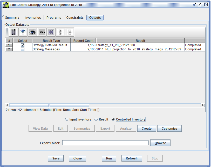
Click the Create button to begin creating the future year inventory. Monitor the Status window for messages and to see when the process is complete.
The future year inventory will automatically be added as a dataset matching the dataset type of the base year inventory. The new dataset’s description will contain comments indicating the strategy used to produce it and the high-level settings for that strategy.
For ORL Inventories:
For the sources that were controlled, CoST fills in the CEFF (control efficiency), REFF (rule effectiveness), and RPEN (rule penetration) columns based on the Control Packets applied to the sources. The CEFF column is populated differently for a replacement Control Packet record than for an add-on Control Packet record. For a replacement control, the CEFF column is populated with the percent reduction of the replacement control. For an add-on control, the CEFF column is populated with the overall combined percent reduction of the add-on control plus the preexisting control, using the following formula:
(1 – {[1 – (existing percent reduction / 100)] x [1 – (add-on percent reduction / 100)]}) x 100
For both types of Control Packet records (add-on or replacement), the REFF and RPEN are defaulted to 100 since the CEFF accounts for any variation in the REFF and RPEN by using the percent reduction instead of solely the CEFF.
Note that only Control Packets (not Plant Closure, Projection, or Allowable packets) will be used to help populate the columns discussed above.
For Flat File 2010 Inventories:
For the sources that were controlled, CoST fills in the annual (ANN_PCT_RED) and monthly percent reduction (JAN_PCT_RED) columns based on the values for the Control Packet that was applied to the sources. The CEFF column is populated differently for a replacement control than for an add-on control. For a replacement control, the CEFF column is populated with the percent reduction of the replacement control. For an add-on control, the CEFF column is populated with the overall combined percent reduction of the add-on control plus the preexisting control, using the following formula:
(1 – {[1 – (existing percent reduction / 100)] x [1 – (add-on percent reduction / 100)]}) x 100
For both types of measures, the REFF and RPEN values are defaulted to 100, because the CEFF accounts for any variation in the REFF or RPEN by using the percent reduction instead of the CEFF.
CoST also populates several additional columns toward the end of the ORL and Flat File 2010 inventory rows that specify information about measures that it has applied. These columns are:
CONTROL MEASURES: An ampersand (&) separated list of control measure abbreviations that correspond to the control measures that have been applied to the given source.
PCT REDUCTION: An ampersand-separated list of percent reductions that have been applied to the source, where percent reduction = CEFF x REFF x RPEN.
CURRENT COST: The annualized cost for that source for the most recent control strategy that was applied to the source.
TOTAL COST: The total cost for the source across all measures that have been applied to the source.
The format of the Plant Closure Packet described in Tbl. 7.6 is based on the CSV format. The first row of this dataset file must contain the column header definition as defined in Line 1 of Tbl. 7.6. All the columns specified here must be included in the dataset import file.
| Line | Position | Description |
|---|---|---|
| 1 | A..H | Column header definition - must contain the following columns: fips,plantid,pointid,stackid,segment,plant,effective_date,reference |
| 2+ | A | Country/State/County code, required |
| B | Plant Id for point sources, optional; blank, zero, or -9 if not specified; leave blank for nonpoint inventories | |
| C | Point Id for point sources, optional; blank, zero, or -9 if not specified; leave blank for nonpoint inventories | |
| D | Stack Id for point sources, optional; blank, zero, or -9 if not specified; leave blank for nonpoint inventories | |
| E | Segment for point sources, optional; blank, zero, or -9 if not specified; leave blank for nonpoint inventories | |
| F | Plant name or description, for point sources, optional; leave blank for nonpoint inventories | |
| G | Effective Date, the effective date for the plant closure to take place. When the closure effective cutoff is after this effective date, the plant will not be closed. A blank value is assumed to mean that the sources matched from this record will be closed regardless. The strategy target year is the year used in the closure effective cutoff date check. See Sec. 7.7.8 for more information. | |
| H | Reference, contains reference information for closing the plant |
The Facility Closure Extended format (Tbl. 7.7) is similar to the Plant Closure Packet but uses column names consistent with the Flat File 2010 inventories. The format also contains additional columns that may be used in the future to further enhance the inventory source matching capabilities: COUNTRY_CD, TRIBAL_CODE, SCC, and POLL.
| Column | Description |
|---|---|
| Country_cd | Country code, optional; currently not used in matching process |
| Region_cd | State/county code, or state code with blank for county, or zero (or blank or -9) for all state/county or state codes |
| Facility_id | Facility ID for point sources, optional; blank, zero, or -9 if not specified; leave blank for nonpoint inventories |
| Unit_id | Unit ID for point sources, optional; blank, zero,or -9 if not specified; leave blank for nonpoint inventories |
| Rel_point_id | Release Point ID for point sources, optional; blank, zero, or -9 if not specified; leave blank for nonpoint inventories |
| Process_id | Process ID for point sources, optional; blank, zero, or -9 if not specified; leave blank for nonpoint inventories |
| Facility_name | Facility name or description, for point sources, optional; leave blank for nonpoint inventories |
| Tribal_code | Tribal code, optional; currently not used in matching process |
| SCC | 8- or 10-digit SCC, optional; blank, zero, or -9 if not an SCC-specific closure; currently not used in matching process |
| Poll | Pollutant name, optional; blank, zero, or -9 if not a pollutant-specific closure; currently not used in matching process |
| Effective_date | Effective Date, the effective date for the plant closure to take place. When the closure effective cutoff is after this effective date, the plant will not be closed. A blank value is assumed to mean that the sources matched from this record will be closed regardless. The strategy target year is the year used in the closure effective cutoff date check. See Sec. 7.7.8 for more information. |
| Comment | Information about this record and how it was produced and entered by the user. |
The format of the Projection Packet (Tbl. 7.8) is based on the SMOKE file format as defined in the SMOKE User’s Manual. One modification was made to enhance this packet’s use in CoST: the unused SMOKE column at position K is now used to store the NAICS code.
| Line | Position | Description |
|---|---|---|
| 1 | A | /PROJECTION <4-digit from year> <4-digit to year>/ |
| 2+ | A | # Header entry. Header is defined by the # as the first character on the line |
| 3+ | A | Country/State/County code, or Country/state code with blank for county, or zero (or blank or -9) for all Country/State/County or Country/state codes |
| B | 8 or 10-digit SCC, optional, blank, zero, or -9 if not a SCC-specific projection | |
| C | Projection factor [enter number on fractional basis; e.g., enter 1.2 to increase emissions by 20%] | |
| D | Pollutant , blank, zero, or -9 if not a pollutant-specific projection | |
| E | Standard Industrial Category (SIC), optional, blank, zero, or -9 if not a SIC- specific projection | |
| F | Maximum Achievable Control Technology (MACT) code, optional, blank, zero, or -9 if not a MACT-specific projection | |
| G | Plant Id for point sources, optional; blank, zero, or -9 if not specified; leave blank for nonpoint inventories | |
| H | Point Id for point sources, optional; blank, zero, or -9 if not specified; leave blank for nonpoint inventories | |
| I | Stack Id for point sources, optional; blank, zero, or -9 if not specified; leave blank for nonpoint inventories | |
| J | Segment for point sources, optional; blank, zero, or -9 if not specified; leave blank for nonpoint inventories | |
| K | North American Industry Classification (NAICS) Code, optional; blank, zero, or -9 if not a NAICS-specific projection | |
| L | Characteristic 5 (blank for ORL inventory input format), optional | |
| 3 | A | /END/ |
The format of the Projection Packet Extended (Tbl. 7.9) dataset is not based on the SMOKE format. It is based on the EMF Flexible File Format, which is based on the CSV-based format. This new format uses column names that are aligned with the Flat File 2010 dataset types in the EMF system. The format also supports monthly projection factors in addition to annual projection factors. For example, instead of using the FIPS code, the new format uses the REGION_CD column, and instead of PLANTID the new format uses FACILITY_ID. The appropriate mapping between the old and new formats is described in Tbl. 7.2. The new format also contains additional columns that will be used in the future to help further enhance the inventory source matching capabilities, these include COUNTRY_CD, TRIBAL_CODE, CENSUS_TRACT_CD, SHAPE_ID, and EMIS_TYPE.
| Column | Description |
|---|---|
| Country_cd | Country code, optional; currently not used in matching process |
| Region_cd | State/county code, or state code with blank for county, or zero (or blank or -9) for all state/county or state codes |
| Facility_id | Facility ID (aka Plant ID in ORL format) for point sources, optional; blank, zero, or -9 if not specified; leave blank for nonpoint inventories |
| Unit_id | Unit ID (aka Point ID for ORL format) for point sources, optional; blank, zero,or -9 if not specified; leave blank for nonpoint inventories |
| Rel_point_id | Release Point ID (aka Stack ID in ORL format) for point sources, optional; blank, zero, or -9 if not specified; leave blank for nonpoint inventories |
| Process_id | Process ID (aka Segment on ORL format) for point sources, optional; blank, zero, or -9 if not specified; leave blank for nonpoint inventories |
| Tribal_code | Tribal code, optional; currently not used in matching process |
| Census_tract_cd | Census tract ID, optional; currently not used in matching process |
| Shape_id | Shape ID, optional; currently not used in matching process |
| Emis_type | Emission type, optional; currently not used in matching process |
| SCC | 8- or 10-digit SCC, optional; blank, zero, or -9 if not an SCC-specific control |
| Poll | Pollutant;, blank, zero, or -9 if not a pollutant-specific projection |
| Reg_code | Regulatory code (aka Maximum Achievable Control Technology code), optional; blank, zero, or -9 if not a regulatory code-specific control |
| SIC | Standard Industrial Category (SIC), optional; blank, zero, or -9 if not an SIC- specific control |
| NAICS | North American Industry Classification (NAICS) code, optional; blank, zero, or -9 if not a NAICS-specific control |
| Ann_proj_factor | The annual projection factor used to adjust the annual emission of the inventory. The number is stored as a fraction rather than a percentage; e.g., enter 1.2 to increase emissions by 20% (double precision). The annual projection factor is also used as a default for monthly-specific projection factors when they are not specified. If you do not want to specify a monthly-specific projection factor value, then also make sure not to specify an annual projection factor, which could be used as a default. |
| Jan_proj_factor | The projection factor used to adjust the monthly January emission of the inventory (the jan_value column of the FF10 inventory). The number is stored as a fraction rather than a percentage; e.g., enter 1.2 to increase emissions by 20% (double precision). If no January projection factor is specified, the annual projection factor value will be used as a default. The monthly-specific projection factor fields are not used on the older ORL inventory formats; only the annual projection factor field will be used on these older formats. |
| Feb_proj_factor | Analogous to the January projections factor, above. |
| … | … |
| Dec_proj_factor | The projection factor used to adjust the monthly December emission of the inventory (the dec_value column of the FF10 inventory). The number is stored as a fraction rather than a percentage; e.g., enter 1.2 to increase emissions by 20% (double precision). If no December projection factor is specified, the annual projection factor value will be used as a default. The monthly-specific projection factor fields are not used on the older ORL inventory formats; only the annual projection factor field will be used on these older formats. |
| Comment | Information about this record and how it was produced and entered by the user. |
The format of the Control Packet (Tbl. 7.10) is based on the SMOKE file format as defined in the SMOKE User’s Manual. Several modifications were made to enhance the packet’s use in CoST:
| Line | Position | Description |
|---|---|---|
| 1 | A | /CONTROL/ |
| 2+ | A | # Header entry. Header is indicated by use of “#” as the first character on the line. |
| 3+ | A | Country/state/county code, or country/state code with blank for county, or zero (or blank or -9) for all country/state/county or country/state codes |
| B | 8- or 10-digit SCC, optional; blank, zero, or -9 if not an SCC-specific control | |
| C | Pollutant; blank, zero, or -9 if not a pollutant-specific control | |
| D | Primary control measure abbreviation; blank, zero, or -9 applies to all measure in the Control Measure Database | |
| E | Control efficiency; value should be a percent (e.g., enter 90 for a 90% control efficiency) | |
| F | Rule effectiveness; value should be a percent (e.g., enter 50 for a 50% rule effectiveness) | |
| G | Rule penetration rate; value should be a percent (e.g., enter 80 for a 80% rule penetration) | |
| H | Standard Industrial Category (SIC); optional, blank, zero, or -9 if not an SIC- specific control | |
| I | Maximum Achievable Control Technology (MACT) code; optional, blank, zero, or -9 if not a MACT-specific control | |
| J | Application control flag: Y = control is applied to inventory N = control will not be used |
|
| K | Replacement flag: A = control is applied in addition to any controls already on source R = control replaces any controls already on the source |
|
| L | Plant ID for point sources, optional; blank, zero, or -9 if not specified; leave blank for nonpoint inventories | |
| M | Point ID for point sources, optional; blank, zero, or -9 if not specified; leave blank for nonpoint inventories | |
| N | Stack ID for point sources, optional; blank, zero, or -9 if not specified; leave blank for nonpoint inventories | |
| O | Segment for point sources, optional; blank, zero, or -9 if not specified; leave blank for nonpoint inventories | |
| P | Compliance Date. The compliance date on which a control can be applied to sources; prior to this date, the control will not be applied. A blank value is assumed to mean that the control is within the compliance date and the sources matched from this record will be controlled regardless. The strategy target year is the year that is used in the control compliance cutoff date check. See Sec. 7.7.8 for more information. | |
| Q | North American Industry Classification (NAICS) Code, optional; blank, zero, or -9 if not a NAICS-specific control | |
| 4 | A | /END/ |
The format of the Control Packet Extended (Tbl. 7.11) dataset is not based on the SMOKE format. It is based on the EMF Flexible File Format, which is based on the CSV-based format. This new format uses column names that are aligned with the Flat File 2010 dataset types in the EMF system. The format also contains additional columns that will be used in the future to help further enhance the inventory source matching capabilities: COUNTRY_CD, TRIBAL_CODE, CENSUS_TRACT_CD, SHAPE_ID, and EMIS_TYPE.
| Column | Description |
|---|---|
| Country_cd | Country code, optional; currently not used in matching process |
| Region_cd | State/county code, or state code with blank for county, or zero (or blank or -9) for all state/county or state codes |
| Facility_id | Facility ID (aka Plant ID in ORL format) for point sources, optional; blank, zero, or -9 if not specified; leave blank for nonpoint inventories |
| Unit_id | Unit ID (aka Point ID for ORL format) for point sources, optional; blank, zero, or -9 if not specified; leave blank for nonpoint inventories |
| Rel_point_id | Release Point ID (aka Stack ID in ORL format) for point sources, optional; blank, zero, or -9 if not specified; leave blank for nonpoint inventories |
| Process_id | Process ID (aka Segment on ORL format) for point sources, optional; blank, zero, or -9 if not specified; leave blank for nonpoint inventories |
| Tribal_code | Tribal code, optional; currently not used in matching process |
| Census_tract_id | Census tract ID, optional; currently not used in matching process |
| Shape_id | Shape ID, optional; currently not used in matching process |
| Emis_type | Emission type, optional; currently not used in matching process |
| SCC | 8- or 10-digit SCC, optional; blank, zero, or -9 if not an SCC-specific control |
| Poll | Pollutant;, blank, zero, or -9 if not a pollutant-specific control |
| Reg_code | Regulatory code (aka Maximum Achievable Control Technology code), optional; blank, zero, or -9 if not a regulatory code-specific control |
| SIC | Standard Industrial Category (SIC), optional; blank, zero, or -9 if not an SIC-specific control |
| NAICS | North American Industry Classification (NAICS) code, optional; blank, zero, or -9 if not a NAICS-specific control |
| Compliance_Date | Compliance Date. The compliance date on which a control can be applied to sources; prior to this date, the control will not be applied. A blank value is assumed to mean that the control is within the compliance date and the sources matched from this record will be controlled regardless. The strategy target year is the year used in the control compliance cutoff date check. See Sec. 7.7.8 for more information. |
| Application_control | Application control flag: Y = control is applied to inventory N = control will not be used |
| Replacement | Replacement flag: A = control is applied in addition to any controls already on source R = control replaces any controls already on the source |
| Pri_cm_abbrev | Primary control measure abbreviation (from the Control Measure Database) that defines the control packet record |
| Ann_pctred | The percent reduction of the control (value should be a percent; e.g., enter 90 for a 90% percent reduction) to apply to the annual emission factor; the percent reduction can be considered a combination of the control efficiency, rule effectiveness, and rule penetration (CE * RE/100 * RP/100). The annual percent reduction field is used to reduce annual emission of the inventory (the ann_value column of the FF10 inventory formats contains the annual emission value). The annual percent reduction is also used as a default for monthly-specific percent reductions when they are not specified. If you do not want to specify a monthly-specific projection factor value, then also make sure not to specify an annual projection factor, which could be used as a default. |
| Jan_pctred | The percent reduction of the control to apply to the monthly January emission factor (the jan_value column of the FF10 inventory). If no January percent reduction is specified, the annual percent reduction value will be used as a default. The monthly-specific percent reduction fields are not used on the older ORL inventory formats; only the annual percent reduction field will be used on these older formats. |
| Feb_pctred | Analogous to the January percent reduction, above. |
| … | … |
| Dec_pctred | The percent reduction of the control to apply to the monthly December emission factor (the dec_value column of the FF10 inventory). If no December percent reduction is specified, the annual percent reduction value will be used as a default. The monthly-specific percent reduction fields are not used on the older ORL inventory formats; only the annual percent reduction field will be used on these older formats. |
| Comment | Information about this record and how it was produced and entered by the user. |
The format of the Allowable Packet (Tbl. 7.12) is based on the SMOKE file format as defined in the SMOKE User’s Manual. Two modifications were made to enhance this packet’s use in CoST:
| Line | Position | Description |
|---|---|---|
| 1 | A | /ALLOWABLE/ |
| 2+ | A | # Header entry. Header is indicated by use of “#” as the first character on the line. |
| 3+ | A | Country/state/county code, or country/state code with blank for county, or zero (or blank or -9) for all country/state/county or country/state codes |
| B | 8- or 10-digit SCC, optional; blank, zero, or -9 if not an SCC-specific cap or replacement | |
| C | Pollutant; blank, zero, or -9 if not a pollutant-specific control; in most cases, the cap or replacement value will be a pollutant-specific value, and that pollutant’s name needs to be placed in this column | |
| D | Control factor (no longer used by SMOKE or CoST; enter -9 as placeholder) | |
| E | Allowable emissions cap value (tons/day) (required if no “replace” emissions are given) | |
| F | Allowable emissions replacement value (tons/day) (required if no “cap” emissions are given) | |
| G | Standard Industrial Category (SIC), optional; blank, zero, or -9 if not an SIC- specific cap or replacement | |
| H | Plant ID for point sources, optional; blank, zero, or -9 if not specified; leave blank for nonpoint inventories | |
| I | Point ID for point sources, optional; blank, zero, or -9 if not specified, leave blank for nonpoint inventories | |
| J | Stack ID for point sources, optional; blank, zero, or -9 if not specified, leave blank for nonpoint inventories | |
| K | Segment for point sources, optional; blank, zero, or -9 if not specified, leave blank for nonpoint inventories | |
| L | Compliance Date. The compliance date on which a cap or replacement entry can be applied to sources; prior to this date, the cap or replacement will not be applied. A blank value is assumed to mean that the cap or replacement is within the compliance date and is available for analysis. See Sec. 7.7.8 for more information. | |
| M | North American Industry Classification (NAICS) Code, optional; blank, zero, or -9 if not a NAICS-specific projection | |
| 4 | A | /END/ |
For control programs that use an effective date (plant closures) or compliance date (controls), CoST uses the control strategy target year to build a cutoff date to use when determining which programs are in effect. To specify the month and day of the cutoff date (used in combination with the target year), there are two EMF system-level properties. These properties are stored in the emf.properties table and are named COST_PROJECT_FUTURE_YEAR_EFFECTIVE_DATE_CUTOFF_MONTHDAY (for effective dates) and COST_PROJECT_FUTURE_YEAR_COMPLIANCE_DATE_CUTOFF_MONTHDAY (for compliance dates). To set a cutoff month/day of October 1, the property value would be “10/01”.
For a strategy with a target year of 2020 and an effective cutoff month/day of 10/01, the closure effective cutoff date is 10/01/2020.
| Closure Record Effective Date | Outcome |
|---|---|
| 07/01/2013 | Effective date is before the cutoff date so all sources matching this record will be closed |
| blank | All sources matching this record will be closed |
| 11/15/2020 | Effective date is after the cutoff date so matching sources will not be closed |
Tbl. 7.13 lists the source matching combinations, the inventory types the matching criteria can be used for, and the Control Program Packet Types that can use these criteria.
| Ranking | Matching Combination | Inventory Types | Control Program Types |
|---|---|---|---|
| 1 | Country/State/County code, plant ID, point ID, stack ID, segment, 8-digit SCC code, pollutant | point | allowable, control, projection, plant closure |
| 2 | Country/State/County code, plant ID, point ID, stack ID, segment, pollutant | point | allowable, control, projection, plant closure |
| 3 | Country/State/County code, plant ID, point ID, stack ID, pollutant | point | allowable, control, projection, plant closure |
| 4 | Country/State/County code, plant ID, point ID, pollutant | point | allowable, control, projection, plant closure |
| 5 | Country/State/County code, plant ID, 8-digit SCC code, pollutant | point | allowable, control, projection, plant closure |
| 6 | Country/State/County code, plant ID, MACT code, pollutant | point | control, projection |
| 7 | Country/State/County code, plant ID, pollutant | point | allowable, control, projection, plant closure |
| 8 | Country/State/County code, plant ID, point ID, stack ID, segment, 8-digit SCC code | point | allowable, control, projection, plant closure |
| 9 | Country/State/County code, plant ID, point ID, stack ID, segment | point | allowable, control, projection, plant closure |
| 10 | Country/State/County code, plant ID, point ID, stack ID | point | allowable, control, projection, plant closure |
| 11 | Country/State/County code, plant ID, point id | point | allowable, control, projection, plant closure |
| 12 | Country/State/County code, plant ID, 8-digit SCC code | point | allowable, control, projection, plant closure |
| 13 | Country/State/County code, plant ID, MACT code | point | control, projection |
| 14 | Country/State/County code, plant ID | point | allowable, control, projection, plant closure |
| 15 | Country/State/County code, MACT code, 8-digit SCC code, pollutant | point, nonpoint | control, projection |
| 16 | Country/State/County code, MACT code, pollutant | point, nonpoint | control, projection |
| 17 | Country/State code, MACT code, 8-digit SCC code, pollutant | point, nonpoint | control, projection |
| 18 | Country/State code, MACT code, pollutant | point, nonpoint | control, projection |
| 19 | MACT code, 8-digit SCC code, pollutant | point, nonpoint | control, projection |
| 20 | MACT code, pollutant | point, nonpoint | control, projection |
| 21 | Country/State/County code, 8-digit SCC code, MACT code | point, nonpoint | control, projection |
| 22 | Country/State/County code, MACT code | point, nonpoint | control, projection |
| 23 | Country/State code, 8-digit SCC code, MACT code | point, nonpoint | control, projection |
| 24 | Country/State code, MACT code | point, nonpoint | control, projection |
| 25 | MACT code, 8-digit SCC code | point, nonpoint | control, projection |
| 26 | MACT code | point, nonpoint | control, projection |
| 27 | Country/State/County code, NAICS code, 8-digit SCC code, pollutant | point, nonpoint | control, projection |
| 28 | Country/State/County code, NAICS code, pollutant | point, nonpoint | control, projection |
| 29 | Country/State code, NAICS code, 8-digit SCC code, pollutant | point, nonpoint | control, projection |
| 30 | Country/State code, NAICS code, pollutant | point, nonpoint | control, projection |
| 31 | NAICS code, 8-digit SCC code, pollutant | point, nonpoint | control, projection |
| 32 | NAICS code, pollutant | point, nonpoint | control, projection |
| 33 | Country/State/County code, NAICS code, 8-digit SCC code | point, nonpoint | control, projection |
| 34 | Country/State/County code, NAICS code | point, nonpoint | control, projection |
| 35 | Country/State code, NAICS code, 8-digit SCC code | point, nonpoint | control, projection |
| 36 | Country/State code, NAICS code | point, nonpoint | control, projection |
| 37 | NAICS code, 8-digit SCC code | point, nonpoint | control, projection |
| 38 | NAICS code | point, nonpoint | control, projection |
| 39 | Country/State/County code, 8-digit SCC code, 4-digit SIC code, pollutant | point, nonpoint | allowable, control, projection |
| 40 | Country/State/County code, 4-digit SIC code, pollutant | point, nonpoint | allowable, control, projection |
| 41 | Country/State code, 8-digit SCC code, 4-digit SIC code, pollutant | point, nonpoint | allowable, control, projection |
| 42 | Country/State code, 4-digit SIC code, pollutant | point, nonpoint | allowable, control, projection |
| 43 | 4-digit SIC code, SCC code, pollutant | point, nonpoint | allowable, control, projection |
| 44 | 4-digit SIC code, pollutant | point, nonpoint | allowable, control, projection |
| 45 | Country/State/County code, 4-digit SIC code, SCC code | point, nonpoint | allowable, control, projection |
| 46 | Country/State/County code, 4-digit SIC code | point, nonpoint | allowable, control, projection |
| 47 | Country/State code, 4-digit SIC code, SCC code | point, nonpoint | allowable, control, projection |
| 48 | Country/State code, 4-digit SIC code | point, nonpoint | allowable, control, projection |
| 49 | 4-digit SIC code, SCC code | point, nonpoint | allowable, control, projection |
| 50 | 4-digit SIC code | point, nonpoint | allowable, control, projection |
| 51 | Country/State/County code, 8-digit SCC code, pollutant | point, nonpoint, onroad, nonroad | allowable, control, projection |
| 52 | Country/State code, 8-digit SCC code, pollutant | point, nonpoint, onroad, nonroad | allowable, control, projection |
| 53 | 8-digit SCC code, pollutant | point, nonpoint, onroad, nonroad | allowable, control, projection |
| 54 | Country/State/County code, 8-digit SCC code | point, nonpoint, onroad, nonroad | allowable, control, projection |
| 55 | Country/State code, 8-digit SCC code | point, nonpoint, onroad, nonroad | allowable, control, projection |
| 56 | 8-digit SCC code | point, nonpoint, onroad, nonroad | allowable, control, projection |
| 57 | Country/State/County code, pollutant | point, nonpoint, onroad, nonroad | allowable, control, projection |
| 58 | Country/State/County code | point, nonpoint, onroad, nonroad | allowable, control, projection, plant closure |
| 59 | Country/State code, pollutant | point, nonpoint, onroad, nonroad | allowable, control, projection |
| 60 | Country/State code | point, nonpoint, onroad, nonroad | allowable, control, projection, plant closure |
| 61 | Pollutant | point, nonpoint, onroad, nonroad | allowable, control, projection |
| Column | Description |
|---|---|
| SECTOR | The source sector specified for the input inventory dataset. |
| CM_ABBREV | For Plant Closure Packets, this column will be set to “PLTCLOSURE”. For Projection Packets, this column will be set to “PROJECTION”. For Control Packets, this column will be set to the abbreviation of the control measure that was applied to the source, if it was explicitly specified in the packet, or it could be the predicted measure abbreviation as found in the CMDB. If no measure can be found, then it will be set to “UNKNOWNMSR”. For Allowable Packets, this column will be set to the predicted abbreviation of the control measure that was applied to the source. If no measure can be found, then it will be set “UNKNOWNMSR”. |
| POLL | The pollutant for the source, found in the inventory |
| SCC | The SCC code for the source, found in the inventory |
| REGION_CD | The state and county FIPS code for the source, found in the inventory |
| FACILITY_ID | For point sources, the facility ID for the source from the inventory. |
| UNIT_ID | For point sources, the unit ID for the source from the inventory. |
| REL_POINT_ID | For point sources, the release point ID for the source from the inventory. |
| PROCESS_ID | For point sources, the process ID for the source from the inventory. |
| ANNUAL_COST ($) | The total annual cost (including both capital and operating and maintenance) required to keep the measure on the source for a year. Note that costs are adjusted to the strategy-defined “Cost Year” dollars. |
| CTL_ANN_COST_PER_TON ($/ton) | This field is not used for the strategy type and is left blank/null. |
| EFF_ANN_COST_PER_TON ($/ton) | The annual cost (both capital and operating and maintenance) to reduce one ton of the pollutant. Note that costs are adjusted to the strategy-defined “Cost Year” dollars. |
| ANNUAL_OPER_MAINT_COST ($) | The annual cost to operate and maintain the measure once it has been installed on the source. Note that costs are adjusted to the strategy-defined “Cost Year” dollars. |
| ANNUAL_VARIABLE_OPER_MAINT_COST ($) | The annual variable cost to operate and maintain the measure once it has been installed on the source. Note that costs are adjusted to the strategy-defined “Cost Year” dollars. |
| ANNUAL_FIXED_OPER_MAINT_COST ($) | The annual fixed cost to operate and maintain the measure once it has been installed on the source. Note that costs are adjusted to the strategy-defined “Cost Year” dollars. |
| ANNUALIZED_CAPITAL_COST ($) | The annualized cost of installing the measure on the source assuming a particular discount rate and equipment life. Note that costs are adjusted to the strategy-defined “Cost Year” dollars. |
| TOTAL_CAPITAL_COST ($) | The total cost to install a measure on a source. Note that costs are adjusted to the strategy-defined “Cost Year” dollars. |
| CONTROL_EFF (%) | The control efficiency as specified by the Control Packet or Allowable Packet. This field is null for Plant Closure and Projection Packets. |
| RULE_PEN (%) | The rule penetration that is specified in the old Control Packet format. For the new Control Extended Packet format, this is set to 100. This field is null for Plant Closure and Projection Packets. |
| RULE_EFF (%) | The rule effectiveness that is specified in the old Control Packet format. For the new Control Extended Packet format, this is set to 100. This field is null for Plant Closure and Projection Packets. |
| PERCENT_REDUCTION (%) | The percent by which the emissions from the source are reduced after the Control Packet has been applied. This field is null for Plant Closure and Projection Packets. |
| ADJ_FACTOR | The adjustment factor stores the Projection Packet factor that is applied to the source. This number is stored in a fractional state rather than as a percentage. This field is null for Plant Closure and Control Packets. |
| INV_CTRL_EFF (%) | The control efficiency for the existing measure on the source, found in the inventory |
| INV_RULE_PEN (%) | The rule penetration for the existing measure on the source, found in the inventory |
| INV_RULE_EFF (%) | The rule effectiveness for the existing measure on the source, found in the inventory |
| FINAL_EMISSIONS (tons) | The final emissions amount that results from the source’s being adjusted by the various Control Program Packets. This is set by subtracting the emis_reduction field by the inv_emissions field. |
| CTL_EMIS_REDUCTION (tons) | This field is not used for the strategy type and is left blank/null. |
| EFF_EMIS_REDUCTION (tons) | This field is used to store the amount by which the emission was reduced for the particular Control Program Packet (Plant Closure, Projection, Control, or Allowable) that is being processed. |
| INV_EMISSIONS (tons) | This field is used to store the beginning/input emission for the particular Control Program Packet (Plant Closure, Projection, Control, or Allowable) that is being processed. |
| APPLY_ORDER | This field stores the Control Program Action Code that is being used on the source. These codes indicate whether the Control Program is applying a Plant Closure, Projection, Control, or Allowable Packet. |
| INPUT_EMIS (tons) | This field is not used for the strategy type and is left blank/null. |
| OUTPUT_EMIS (tons) | This field is not used for the strategy type and is left blank/null. |
| FIPSST | The two-digit FIPS state code. |
| FIPSCTY | The three-digit FIPS county code. |
| SIC | The SIC code for the source from the inventory. |
| NAICS | The NAICS code for the source from the inventory. |
| SOURCE_ID | The record number from the input inventory for this source. |
| INPUT_DS_ID | The numeric ID of the input inventory dataset (for bookkeeping purposes). |
| CS_ID | The numeric ID of the control strategy |
| CM_ID | This field is not used for the strategy type and is left blank/null. |
| EQUATION TYPE | The control measure equation that was used during the cost calculations. If a minus sign is in front of the equation type, this indicates that the equation type was missing inputs and the strategy instead used the default approach to estimate costs. Note that this field will be used only when Control Packets are applied, not when any of the other packet types are applied. |
| ORIGINAL_DATASET_ID | This field is not used for the strategy type and is left blank/null. |
| SECTOR | This field is not used for the strategy type and is left blank/null. |
| CONTROL_PROGRAM | The control program that was applied to produce this record |
| XLOC | The longitude for the source, found in the inventory for point sources, for nonpoint inventories the county centroid is used. This is useful for mapping purposes |
| YLOC | The latitude for the source, found in the inventory for point sources, for nonpoint inventories the county centroid is used. This is useful for mapping purposes. |
| FACILITY | The facility name from the inventory (or county name for nonpoint sources) |
| REPLACEMENT_ADDON | Indicates whether the Control Packet was applying a replacement or an add-on control. A = Add-On Control R = Replacement Control Note that this field will be used only when Control Packets are applied, not when any of the other packet types are applied. |
| EXISTING_MEASURE_ABBREVIATION | This field is not used for the strategy type and is left blank/null. |
| EXISTING_PRIMARY_DEVICE_TYPE_CODE | This field is not used for the strategy type and is left blank/null. |
| STRATEGY_NAME | This field is not used for the strategy type and is left blank/null. |
| CONTROL_TECHNOLOGY | This field is not used for the strategy type and is left blank/null. |
| SOURCE_GROUP | This field is not used for the strategy type and is left blank/null. |
| COUNTY_NAME | This field is not used for the strategy type and is left blank/null. |
| STATE_NAME | This field is not used for the strategy type and is left blank/null. |
| SCC_L1 | This field is not used for the strategy type and is left blank/null. |
| SCC_L2 | This field is not used for the strategy type and is left blank/null. |
| SCC_L3 | This field is not used for the strategy type and is left blank/null. |
| SCC_L4 | This field is not used for the strategy type and is left blank/null. |
| JAN_FINAL_EMISSIONS | The monthly January final emission that results from the source’s being adjusted by the various Control Program Packets. This is set by subtracting the monthly January emission reduction by the monthly January input emission. This monthly- related field is populated only when projecting Flat File 2010 inventories. |
| FEB_FINAL_EMISSIONS | Same as defined for the jan_final_emissions field but for February. |
| … | … |
| DEC_FINAL_EMISSIONS | Same as defined for the jan_final_emissions field but for December. |
| JAN_PCT_RED | The percent by which the source’s January monthly emission is reduced after the Control Packet has been applied. This field is null for Plant Closure and Projection Packets. This monthly-related field is only populated when projecting Flat File 2010 inventories. |
| FEB_PCT_RED | Same as defined for the jan_pct_red field but for February |
| … | … |
| DEC_PCT_RED | Same as defined for the jan_pct_red field but for December |
| COMMENT | Information about this record and how it was produced; this can be either created automatically by the system or entered by the user. |
| Column | Description |
|---|---|
| Fips | The state and county FIPS code for the source, found in the inventory |
| Scc | The SCC code for the source, found in the inventory |
| PlantId | For point sources, the plant/facility ID for the source, found in the inventory |
| PointId | For point sources, the point/unit ID for the source, found in the inventory |
| StackId | For point sources, the stack/release point ID for the source, found in the inventory |
| Segment | For point sources, the segment/process ID for the source, found in the inventory |
| Poll | The pollutant for the source, found in the inventory |
| Status | The status type. The possible values are listed below: Warning - description Error - description Informational - description |
| control_program | The control program for the strategy run; this is populated only when using the PFYI strategy type. |
| message | The text describing the strategy problem. |
| message_type | Contains a high-level message-type category. Currently this is populated only when using the PFYI strategy type. The possible values are listed below: Inventory Level (or blank) - message has to do specifically with a problem with the inventory Packet Level - message has to do specifically with a problem with the packet record being applied to the inventory |
| inventory | Identifies the inventory with the problem. |
| Packet_fips | The state and county FIPS/region code for the source, found in the control program packet |
| Packet_scc | The SCC code for the source, found in the control program packet |
| Packet_plantId | For point sources, the plant/facility ID for the source, found in the control program packet |
| Packet_pointId | For point sources, the point/unit ID for the source, found in the control program packet |
| Packet_stackId | For point sources, the stack/release point ID for the source, found in the control program packet |
| Packet_segment | For point sources, the segment/process ID for the source, found in the control program packet |
| Packet_poll | The pollutant for the source, found in the control program packet |
| Packet_sic | The SIC code for the source, found in the control program packet |
| Packet_mact | The MACT/regulatory code for the source, found in the control program packet |
| Packet_naics | The NAICS code for the source, found in the control program packet |
| Packet_compliance_effective_date | The compliance or effective date, found in the control program packet. The compliance date is used in the Control Packet; the effective date is used in the Plant Closure Packet |
| Packet_replacement | Indicates whether the packet identifies a replacement versus an add-on control, found in the control program packet |
| Packet_annual_monthly | Indicates whether the packet is monthly based or annual based |
The “module type” and “module” features have been developed as a component of the EMF and reuse many of its features (dataset types, datasets, client-server architecture, PostgreSQL database, etc.), while allowing users flexibility to utilize datasets in new ways through PostgreSQL commands.
Both “module types” and “modules” are easy to use and are flexible enough to address a wide variety of scenarios, systematically tracks changes in either algorithms, inputs or assumptions; moreover, these changes are easy to document.
A module type defines an algorithm which can operate on input datasets and parameters and produces output datasets and parameters. Module types are equivalent to functions in most programming languages.
A simple module type implements the algorithm in PL/pgSQL, the SQL procedural language for the PostgreSQL database system. A composite module type implements the algorithm using a network of interconnected submodules based on other (simple or composite) module types.
A module is a construct that binds a module type’s inputs and outputs to concrete datasets and parameter values. Running a module executes the algorithm on the concrete datasets and parameter values bound to inputs and produces the datasets and parameters bound to outputs. Modules are equivalent to complete executable programs.
The module types and the modules are generic components and can be used to implement any model.
The module type and module features consist of:
A module’s outputs can be another module’s inputs. Consequently, the modules can be organized in complex networks modeling complex dataflows.
The relationship between Module Types and Modules is very similar to the relationship between Dataset Types and Datasets:
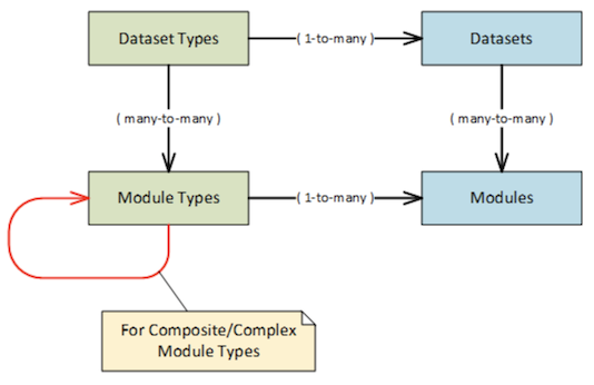
The Module Type Manager window lists the existing module types and allows the user to view edit, create, or remove module types. The user can create simple or composite module types.
Removing module types used by modules and other module types requires user confirmation:
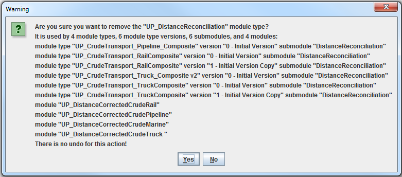
Only users with administrative privileges can remove entire module types via the Module Type Manager window.
The Module Type Version Manager window lists all module type versions for the selected module type and allows the user to view, edit, copy, and remove module type versions. Only users with administrative privileges can remove module type versions that have been finalized.
The Module Type Version Properties window lists module type metadata (name, description, creator, tags, etc.), module type version metadata (version, name, description, etc.), datasets, parameters, and revision notes for the selected module type version. It also lists the algorithm for simple module types and the submodules and the connections for the composite module types. The user can select a parameter’s type from a limited (but configurable) list of SQL types (integer, varchar, etc.).
The user can indicate that a dataset or parameter is optional. For composite module types, if the target of a connection is optional then a source does not have to be selected. The UI prevents the user from connecting an optional source to a non-optional (required) target.
The algorithm for a simple module type must handle optional datasets and parameters. The following placeholders (macros) can be used to test if a dataset/parameter is optional and if a dataset/value was provided: ${placeholder-name.is_optional}, ${placeholder-name.is_set}, #{parameter-name.is_optional}, and #{parameter-name.is_set}. See Algorithm Syntax (Sec. 8.5).
The user can change, save, validate, and finalize the module type version. The user is automatically prompted to add new revision notes every time new changes are saved. The validation step verifies (among other things) that all dataset placeholders in the algorithm are defined.
Updating a module type version used by modules and other composite module type versions requires user confirmation:
For a composite module type, finalizing a module type version requires finalizing all module type versions used by submodules, recursively. The user is shown the list of all required changes and the finalization proceeds only after the user agrees to all the changes.
When working with a composite module type, the Diagram tab displays a diagram illustrating the composite module type’s submodules, inputs, outputs, and connections. Each submodule is color-coded so that the submodule and its specific inputs and outputs can be identified. Overall inputs to the composite module type are shown with a white background. In the diagram, datasets are identified by boxes with blue borders, and dataset connection are shown with a blue line. Parameters use boxes with red borders, and parameter connections use red lines.
The Module Manager UI that lists the existing modules and allows the user to view, edit, create, copy, remove, compare, and run modules.
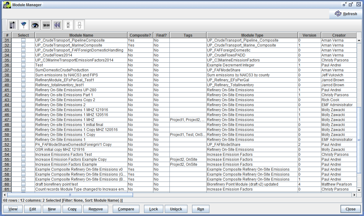
Users who do not have administrative privileges can only remove modules that they created, and only modules that have not been finalized. When removing a module, the user can choose to remove all datasets that were output by that module. Datasets that are used as inputs to other modules, or are in use by other parts of the EMF (e.g. control strategies, control programs) won’t be deleted. Eligible output datasets will be fully deleted, the equivalent of Remove and Purge in the Dataset Manager.
The module comparison feature produces a side-by-side report listing all module attributes and the comparison results: MATCH, DIFFERENT, FIRST ONLY, SECOND ONLY.
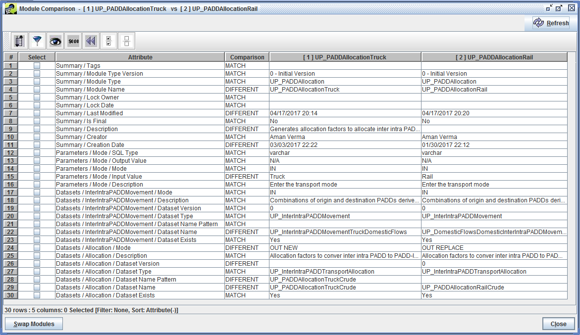
The View/Edit Module window lists metadata (description, creator, tags, project, etc.), dataset bindings, parameter bindings, and execution history for the selected module. The user can bind concrete datasets to dataset placeholders and concrete values to input parameters. If a dataset/parameter is optional then a dataset/value binding is not required.
The View/Edit Module window also lists the algorithm for simple module types and the submodules, connections, internal datasets, and internal parameters for composite module types. The internal datasets and parameters are usually lost after a run, but the user can choose to keep some or all internal datasets and parameters (mostly for debugging). The user can change, save, validate, run, and finalize the selected module.
In the datasets tab the user can select and open a concrete dataset used or produced by the run (if any) and inspect the data. The user can also obtain the list of modules related to a concrete dataset. A module is related to a dataset if it produced the dataset as output or it’s using the dataset as input.
In the parameters tab the user can inspect the value of the output parameters as produced by the last run (only if the last run was successful).
A module can be finalized if the following conditions are met:
Finalizing a module finalizes the input and output datasets also.
The View/Edit Module window has a status indicator that informs the user that the module is UpToDate or OutOfDate.
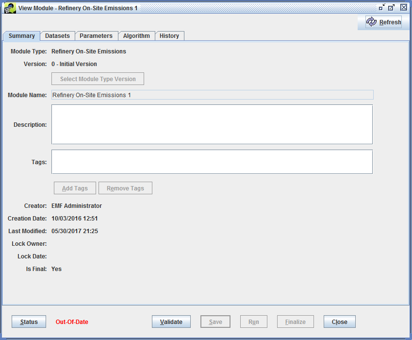
The Status button brings up a dialog box explaining why the module is Out-Of-Date.
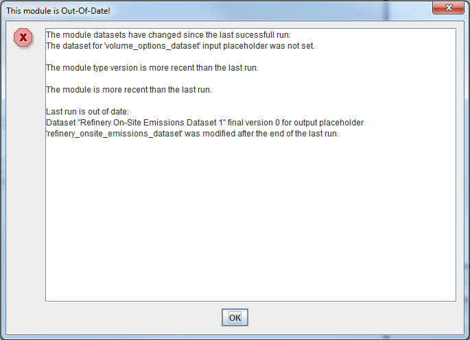
A module is UpToDate when:
The Module History window lists all execution records for the selected module. The user can select and view each record in the Module History Details window.
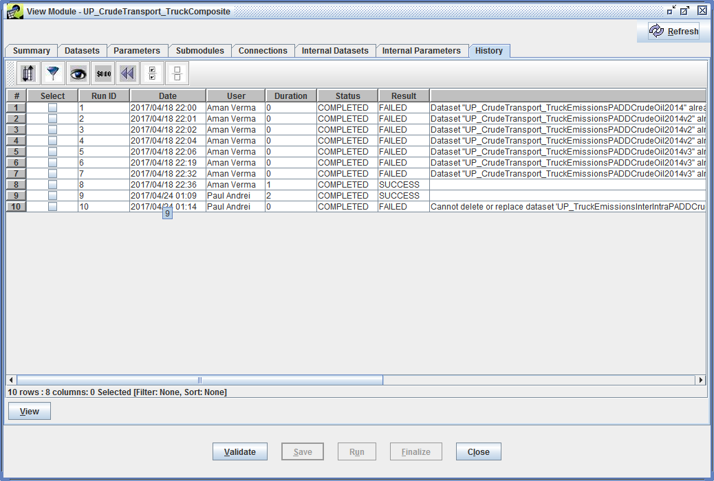
The Module History Details window lists metadata, concrete datasets used or produced by the run (including the internal datasets the user chose to keep), the parameter values used or produced by the run (including the internal parameters the user chose to keep), the actual setup/user/teardown scripts executed by the database server for the module and each submodule, and detailed logs including error messages, if any. The user can select and open a concrete dataset used or produced by the run and inspect the data. The user can also obtain the list of modules related to a concrete dataset.
The setup script used by the Module Runner creates a temporary database user with very limited permissions. It also creates a temporary default schema for this user.
The actual user scripts executed by the database server for each simple module or submodule contains the algorithm (with all placeholders replaced) surrounded by some wrapper/interfacing code generated by the Module Runner. The user script is executed under the restricted temporary database user account in order to protect the database from malicious or buggy code in the algorithm.
The teardown script drops the temporary schema and the temporary database user.
The Dataset Manager lists all datasets in the EMF, including those used by modules, with options to view, edit, import, export, and remove datasets. When removing a dataset via the Dataset Manager, the system checks if that dataset is in use by a module as 1) an input to a module, 2) an output of a module where the module replaces the dataset, or 3) the most recent output created as a new dataset from a module. If any of the usage conditions are met, the dataset will not be deleted; the Status window will include a message detailing which modules use which datasets.
The Simple Module Runner is a server component that validates the simple module, creates the output datasets, creates views for all datasets, replaces all placeholders in the module’s algorithm with the corresponding dataset views, executes the resulting scripts on the database server (using a temporary restricted database user account), retrieves the values of all output parameters, and logs the execution details including all errors, if any. The Module Runner automatically adds new custom keywords to the output datasets listing the module name, the module database id, and the placeholder.
The Composite Module Runner is a server component that validates the composite module and executes its submodules in order of dependencies by:
The order in which the submodules are executed is repeatable: when multiple submodules independent of each other are ready for execution, they are processed in the order of their internal id.
The Composite Module Runner keeps track of temporary internal datasets and parameters and deletes them as soon as they are not needed anymore, unless the user explicitly chose to keep them.
While running a module, the Module Runner enforces strict dataset replacement rules to prevent unauthorized dataset replacement.
The algorithm for a simple module type must be written in PL/pgSQL, the SQL procedural language for the PostgreSQL database system (https://www.postgresql.org/docs/9.5/static/plpgsql-overview.html).
The EMF Module Tool extends this language to accept placeholders for the module’s datasets. The placeholder syntax is: ${placeholder-name}. For example, if a module type has defined a dataset called input_options_dataset then the algorithm can refer to it using the ${input_options_dataset} syntax.
The module tool also uses placeholders for the module’s parameters. The parameter placeholder syntax is: #{parameter-name}. For example, if a module type has defined a parameter called increase_factor then the algorithm can refer to it using the #{increase_factor} syntax.
For example, the following algorithm reads records from input_emission_factors_dataset, applies a multiplicative factor to the Emission_Factor column, and inserts the resulting records into a new dataset called output_emission_factors_dataset:
INSERT INTO ${output_emission_factors_dataset}
    (Fuel_Type, Pollutant, Year, Emission_Factor, Comments)
SELECT
    ief.Fuel_Type,
    ief.Pollutant,
    ief.Year,
    ief.Emission_Factor * #{increase_factor},
    ief.Comments
FROM ${input_emission_factors_dataset} ief;
More detailed information is available for each dataset placeholder:
| Placeholder | Description | Example |
|---|---|---|
| ${placeholder-name.table_name} | The name of the PostgreSQL table that holds the data for the dataset. | emissions.ds_inputoptions_dataset_1_1165351574 |
| ${placeholder-name.dataset_name} | The dataset name. | Input Options Dataset |
| ${placeholder-name.dataset_id} | The dataset id. | 156 |
| ${placeholder-name.version} | The version of the dataset as selected by the user. | 2 |
| ${placeholder-name.view} | The name of the temporary view created for this dataset table by the Module Runner. | input_options_dataset_in_view |
| ${placeholder-name} | Same as ${placeholder-name.view}. | input_options_dataset_in_view |
| ${placeholder-name.mode} | The dataset mode: IN, INOUT, or OUT, where IN is an input dataset, INOUT is both an input and updated as output, and OUT is an output dataset. | IN |
| ${placeholder-name.output_method} | The dataset output method (defined only when mode is OUT): NEW or REPLACE. | NEW |
| ${placeholder-name.is_optional} | TRUE if the dataset is optional, FALSE if the dataset is required | TRUE |
| ${placeholder-name.is_set} | TRUE if a dataset was provided for the placeholder, FALSE otherwise | TRUE |
The following “general information” placeholders related to the current user, module, or run are defined also:
| Placeholder | Description | Example |
|---|---|---|
| ${user.full_name} | The current user’s full name. | John Doe |
| ${user.id} | The current user’s id. | 6 |
| ${user.account_name} | The current user’s account name. | jdoe |
| ${module.name} | The current module’s name. | Refinery On-Site Emissions |
| ${module.id} | The current module’s id. | 187 |
| ${module.final} | If the module is final, then the placeholder is replaced with the word Final. Otherwise the placeholder is replaced with the empty string. | Final |
| ${module.project_name} | If the module has a project, then the placeholder is replaced with the name of the project. Otherwise the placeholder is replaced with the empty string. | |
| ${run.id} | The unique run id. | 14 |
| ${run.date} | The run start date. | 11/28/2016 |
| ${run.time} | The run start time. | 14:25:56.825 |
The following parameter placeholders are defined:
| Placeholder | Description | Example |
|---|---|---|
| #{parameter-name} | The name of the parameter with a timestamp appended to it. | increase_factor_094517291 |
| #{parameter-name.sql_type} | The parameter’s SQL type. | double precision |
| #{parameter-name.mode} | The parameter mode: IN, INOUT, or OUT, where IN is an input parameter, INOUT is both an input and updated as output parameter (e.g. an index value), and OUT is an output parameter. | IN |
| #{parameter-name.input_value} | The parameter’s input value (defined only when mode is IN or INOUT). | 1.15 |
| #{parameter-name.is_optional} | TRUE if the parameter is optional, FALSE if the parameter is required | TRUE |
| #{parameter-name.is_set} | TRUE if a value was provided for the parameter, FALSE otherwise | TRUE |
The “general information” placeholders listed above (see Tbl. 8.2) can also be used to build output dataset name patterns in the Module Editor. For example, a module could specify the following name pattern for a new output dataset:
Refinery On-Site Emissions #${run.id} ${user.full_name} ${run.date} ${run.time}
When running the module, all placeholders in the name pattern will be replaced with the corresponding current value. For example:
Refinery On-Site Emissions #43 John Doe 12/05/2016 09:45:17.291
Problem:
On startup, an error message is displayed like Fig. 9.1:
"The EMF client was not able to contact the server due to this error:
(504)Server doesn’t respond at all."
or
(504)Server denies connection.
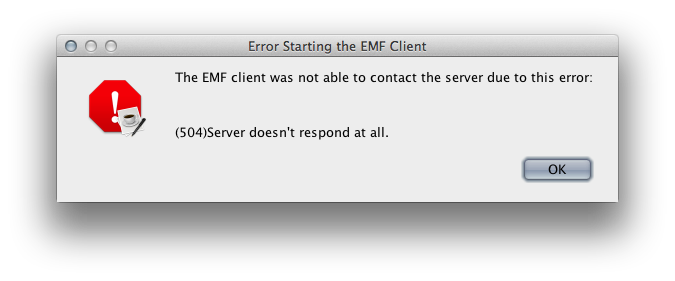
Solution:
The EMF client application was not able to connect to the EMF server. This could be due to a problem on your computer, the EMF server, or somewhere in between.
If you are connecting to a remote EMF server, first check your computer’s network connection by loading a page like google.com in your web browser. You must have a working network connection to use the EMF client.
Next, check the server location in the EMF client start up script C:\EMF_State\EMFClient.bat. Look for the line
set TOMCAT_SERVER=http://<server location>:8080
You can directly connect to the EMF server by loading
http://<server location>:8080/emf/services
in your web browser. You should see a response similar to Fig. 9.2.
If you can’t connect to the EMF server or don’t get a response, then the EMF server may not be running. Contact the EMF server administrator for further help.
Problem:
When I click the Datasets item from the main Manage menu, nothing happens and I can’t click on anything else.
Solution:
Clicking Datasets from the main Manage menu displays the Dataset Manager. In order to display this window, the EMF client needs to request a complete list of dataset types from the EMF server. If you are connecting to an EMF server over the Internet, fetching lists of data can take a while and the EMF client needs to wait for the data to be received. Try waiting to see if the Dataset Manager window appears.
Problem:
In the Dataset Manager, I selected Show Datasets of Type “All” and nothing happens and I can’t click on anything else.
Solution:
When displaying datasets of the selected type, the EMF client needs to fetch the details of the datasets from the EMF server. If you are connecting to an EMF server over the Internet or if there are many datasets imported into the EMF, loading this data can take a long time. Try waiting to see if the list of datasets is displayed. Rather than displaying all datasets, you may want to pick a single dataset type or use the Advanced search to limit the list of datasets that need to be loaded from the EMF server.
The EMF server consists of a database, file storage, and the server application which handles requests from the clients and communicates with the database.
The database server is PostgreSQL version 9.2 or later. For ShapeFile export, you will need the PostGIS module installed.
The server application is a Java executable that runs in the Apache Tomcat servlet container. You will need Apache Tomcat 8.0 or later.
The server components can run on Windows, Linux, or Mac OS X.
The EMF client application communicates with the server on port 8080. For the client application, the EMFClient.bat launch script specifies the server location and port via the setting
set TOMCAT_SERVER=http://<server address>:8080
In order to import data into the EMF, the files must be locally accessible by the server. Depending on your setup, you may want to mount a network drive on the server or allow SFTP connections for users to upload files.
Inside the EMF client, users with administrative privileges have access to additional management options.
EMF administrators can reset users passwords. Administrators can also create new users.
Administrators can create and edit dataset types. Administrators can also add QA step templates to dataset types.