The Models-3/EDSS I/O API is intended to provide an easy-to-learn, easy-to-use interface to data files for the model and model-related-tool developer, together with utility routines for a variety of needed modeling tasks, and a selection of m3tools related programs.There are only a few topics you'll need to know about:
- Files, Logical Names and Physical Names
- File descriptions, and types of data supported
- How to start up and shut down the I/O API
- How to open or create files
- How to read data from files
- How to write data to files
- Date and Time Conventions
- Grid and Coordinate System Conventions
- Other Useful Capabilities
- EXAMPLE: Typical Modeling Program
- I/O API Programmers Manual
The Models-3 Input/Output Applications Programming Interface (I/O API) is a selective and direct-access programming interface to the data: you tell the system what variables and dates and times you're talking about and it figures all the stuff about record numbers, etc., for itself. Also, you don't have to read the data in consecutive order, or to write it in order, either -- you just ask for what you want, and the I/O API finds it for you (although there are moderate performance penalties for writing data out-of-order). The files are self-describing files -- that is, the file headers have all the dimensioning and descriptive information needed about the data in them.There is an underlying object model for environmental data (especially atmospheric data) and the models that use it — see the Requirements Document for more detail. In general, if you're wondering about how to manipulate the underlying objects according to the I/O API conventions, there is probably an I/O API routine or m3tools. program already written to do it for you.
On the other hand, a number of people have attempted to "get around" the API and treat it as a "data format", reading or writing its data directly with their programs (e.g., PAVE and VERDI). So far, every one of these attempts has screwed up to one degree or another.There are versions of the I/O API callable from both Fortran and from C. This document describes the Fortran interface; the C interface is very similar. The major difference between the two are that Fortran LOGICAL functions returning .TRUE. or .FALSE. correspond to C functions returning 1 or 0, Fortran
".EXT"include-files correspond one-to-one to C".h"include files, and the C calls look much like the Fortran calls, except that file descriptions are passed via pointers to data structures typedeffed in fdesc3.h instead of aCOMMONfound inFDESC3.EXTFor Fortran programmers,
MODULE
    M3UTILIO
provides not only the contents of theseINCLUDE-files but also declarations and explicit interfaces (that allow the compiler to check that subroutine calls get their argument-lists correct) for almost all the I/O API routines. It is strongly suggested that youUSEthisMODULE, rather than including theINCLUDE-files directly.There are 9 fundamental I/O routines you'll need to know; these are described in more detail in later sections of the documentation. (In all, there are about 200 Fortran and 60 C routines, many of which are "private" routines used internally. See the I/O API Programmers Manual.)
There is one master Fortran-90
INIT3()to start up (returning the Fortran unit number for the log file; it may be called repeatedly, and is a "no-op" for such repeated calls);M3EXIT(), to shut programs down properly; it flushes all files, generates exit messages to the program log and then terminates the program with a user-supplied exit status (which should be 0 for success and nonzero for failure).
This is a requirement for proper process management.OPEN3()to open files;DESC3()to get file descriptions;READ3(),INTERP3(),XTRACT3(), andDDTVAR3()to read, read-and-time-interpolate, or read-and-time-derivative data from files, respectively; andWRITE3()to store data to files.MODULE,MODULE M3UTILIO, which provides declarations and Fortran-90INTERFACEs for the routines, as well as incorporating threeINCLUDEfiles you'll have to worry about:Each of these
- PARMS3.EXT for Fortran and parms3.h for C
- contain the dimensioning parameters and the "magic number" parameters used to control the operation of various routines in the I/O API;
- FDESC3.EXT for Fortran and fdesc3.h for C
- have
COMMONs orstructs that hold file descriptions (more about that later); FDESC3.EXT needs PARMS3.EXT for its own dimensioning; and
- IODECL3.EXT for Fortran and iodecl3.h for C
- have declarations and usage comments for the various functions in the I/O API (really a short manual on the I/O API in its own right).
iodecl3.h automatically #includes both parms3.h and fdesc3.h
INCLUDE-files has extensive in-line documentation describing how it is used.Normally, Fortran routines that use the I/O API should begin as follows, to define all these declarations,
PARAMETERs andINTERFACEs:... USE M3UTILIO ...C codes should similarly... #include "iodecl3.h" ...
The I/O API stores and retrieves data using files and virtual files, which have (optionally) multiple time steps of multiple layers of multiple variables. Files are formatted internally so that they are machine and network-independent—you can FTP them freely across a wide variety of machines, or read files NFS-mounted from other machines, as well. (This behavior is unlike Fortran files, whose internal formats are vendor specific, so that the files don't FTP or NFS-mount very well, and aren't even necessarily compatible from compiler-version to compiler version). Each file has an internal description, consisting of the file type, the grid and coodinate descriptions, a set of descriptions for the file's set of variables, i.e., names, units specifications, and text descriptions. Each variable has a set of layers and a sequence of time steps (quite possibly only one layer for some kinds of data, if you want, or only one time step, for time-independent data). In dealing with the files, we'll refer to files and variables by names, layers by number (from 1 to the number of layers in the file), and dates and times according to conventions described later. Rather than forcing the programmer and program-user to deal with hard-coded file names or hard-coded unit numbers, the I/O API introduces the concept of logical file names. As a modeler, you can define your own logical names as properties of a program (or even prompt the user for his own preferred logical names at run time) and then at run-time connect up the logical names to any "real" file name you want to, using the UNIX csh setenv command. Additionally, there are four standard logical names:For programming purposes, the significant facts are that names should not contain arithmetic operations (
- LOGFILE for the program log file (if desired);
- SCENFILE for the scenario (run-) description file;
- EXECUTION_ID for a one-line-text run-description/identifier; and
- GRIDDESC, for the ASCII grid and coordinate system databases used by utility routine
DSCGRID().+-*/), or blanks (except at the end:"foo "is OK;"f oo"is not), and are at most 16 characters long.When you run a program that uses the I/O API, you begin with the sequence of setenv commands that set the values for the program's logical names, much as you begin a (normal) Cray Fortran program with a sequence of ASSIGN commands for its files. For example, if "myprogram" has logical names "foo" and "bar" that I want to connect up to files "somedata.mymodel" and "otherdata.whatever" from directory "/tmp/mydir", the script for the program would look something like:
    ...
    setenv foo          /tmp/mydir/somedata.mymodel
    setenv bar          /tmp/mydir/otherdata.whatever
    setenv qux         "/tmp/mydir/volatilestuff.mymodel -v"
    setenv LOGFILE      /tmp/mydir/mymodel.log
    setenv SCENFILE     /tmp/mydir/test17a.description
    setenv EXECUTION_ID TEST17A
    /user/mydir/myprogram
    ...
PnetCDF/MPI distributed files are indicated by a leadingMPI:prefix, e.g.,setenv foo MPI:/tmp/mydir/somedata.mymodelNative-binary files (For NCEP) are indicated by a leading
BIN:prefix, e.g.,setenv bar BIN:/tmp/mydir/somedata.mymodelVOLATILE files are indicated by a trailing
-vin the setenv command, as above, in order to tell the I/O API to perform disk-synch operations before every input and after every output operation on that file. Such files can be accessed by other programs while the generating program is still running, and are readable even if it fails to do a SHUT3() or M3EXIT(), or if the program crashes unexpectedly).BUFFERED virtual files can be used to provide safe, structured exchange of data — of "gridded", "boundary", or "custom" types only — between different modules in the same program. If you
setenvthe value of a logical name to the valueBUFFERED, as given below:... setenv qux BUFFERED ... /user/mydir/myprogram ...then the I/O API will establish in-memory buffers and time indexing for "qux" instead of creating a physical file on disk. One module can then useWRITE3()(see below) to export data for sharing, which other modules would then useREAD3()orINTERP3()to import. Note that since these routines associate the data with its simulation date-and-time, the system will notice the error (and warn the user) if you attempt to get and use data before it has been produced. Note also that by changing the setenv in the script between "BUFFERED" and a physical file-name, you can change between efficient data sharing between modules and high-resolution instrumentation of the data being shared, without changing the underlying program at all.COUPLING-MODE virtual files can be used to provide PVM-based data exchange between cooperating programs using exactly the unchanged I/O API programming interface, with the kind of name-based direct-access semantics that provides, with the extra scheduling condition that requests for data that has not yet been written put the requester to sleep until it becomes available (at which time the requester is awaked and given the requested data). The decision of which files are disk-based and which are COUPLING-MODE virtual files is also made by setenv commands at program-launch, the value being of the form
virtual <communications-channel-name>orPVM:<communications-channel-name>as in one of the following:... setenv qux PVM:CHEM_CONC_2D_G3 setenv zok "virtual CHEM_CONC_3D_G3" /user/mydir/myprogram ...Except for
INIT3()(which returns the Fortran unit number for the log file), all of the fundamental I/O API routines areLOGICALfunctions returningTRUEfor success andFALSEfor failure.There are a number of dimensioning parameters and "magic number" token values for the I/O API. Throughout the I/O API, names (logical file names, variable names, and units) are character strings with maximum length
NAMLEN3 = 16; descriptions are either one orMXDESC3 = 60lines of length at mostMXDLIN3 = 80. The I/O API currently supports up to MXFILE3 = 64 open files, each with up toMXVARS3 = 2048variables (MXVARS3 = 120for I/O API version 3.0 or earlier).
The include-files FDESC3.EXT for Fortran, and fdesc3.h for C contain heavily annotated declarations for all the variables in a file description, together with the two commons which are used by the I/O API to store and retrieve the file descriptions. TheDESC3()routine takes a file and puts its description into theFDESC3 COMMONs;OPEN3()does roughly the reverse when dealing with new or unknown files, taking a description from theFDESC3commons and building a new file according to those specifications, or performing a consistency check with the description stored in the file's header if the file already exists. A typical call toDESC3()might look like:.. IF ( .NOT. DESC3( 'myfile' ) ) THEN ...(error: probably the file hasn't been opened yet) END IFSome of the items in a file description, such as the dates and times for file creation and update, and the name of the program which created the file, are maintained automatically by the system. Others describe the variables in the file: the file type (as described above), the number of variables, their names, unit designations, and descriptions, as well as the description of the file as a whole. Still others dimension the data: the number of layers and the grid dimensions (where for ID and profile files, the number of sites is mapped onto the rows dimension; for profile files, the number of vertical levels is mapped onto the columns dimension). Still other parts of the file description specify the geometry of the grid: the map projection used, its projection parameters, and the grid's location and cell-size relative to that map projection; the vertical-grid-coordinate type and the boundary values separating the model layers.All files manipulated by the I/O API have multiple variables, each having possibly multiple layers. Within a file, all the variables are data arrays have the same dimensions, number of layers and the same structure-type of data, although possibly different basic types (e.g., gridded and boundary varaibles can't be mixed within the same file, but real and integer variables can). Each file has a time step structure shared by all of its variables, as well. There are three kinds of time-step structure supported:
NOTE 1: this is designed to support very-long time step sequences: the author has performed 33-year runs with time steps as small as 30 minutes (over 500,000 time steps), and the access methods are designed to support analysis and visualization of such large (>3TB) data sets.
- Time-independent. The file's time-step attribute is set to zero.
Routines which deal with time-independent files ignore the date and time arguments.- Time-stepped. The file has a starting date, a starting time, and a positive time step. Read and write requests must be for some positive integer multiple of the time step from the starting date and time, or they will fail.
- Circular-buffer. The file keeps only two "records", the "even" part and the "odd" part (useful, for example, for "restart" files where you're only interested in the last good data in the file). The file's description has a starting date, a starting time, and a negative time step (set to the negative of the actual time step); read and write requests must be for some positive integer multiple of the time step from the starting date and time -- and must be for a time step actually present -- or they will fail.
NOTE 2: By convention, standard-year and standard-week data are represented by using year 0:
for example, if one has monthly standard year data, one may store the data in a file starting at Dec. 16 of Year -1 (JDATE=-650=-1000+350, whereYYYY=(-1000), DDD=350), with time step 7300000 (30 days, 10 hours) and 14 time-steps (for December of Year (-1) through January of Year 1), to provide "fenceposts" for daily or hourly interpolation usingINTERP3().
Similarly, a standard-week file might have starting date&time 0000001:000000, time step 240000 (one day), and 7 time steps; one would then useCURRSTEP()(described below) to determine dates and times forREAD3().There are eight structure-types and four basic types of data supported by the I/O API. The structure-types are associated with file type parameter values ("magic numbers")
(for which
CUSTOM3, for single-indexed array with meaning to be defined by the user;DCTNRY3, for file-dictionary (not currently used);GRDDED3, for gridded data;BNDARY3, for grid-boundary data;IDDATA3, for ID-referenced (e.g., observational) data;PROFIL3, for observational vertical-profile (e.g., rawindsonde) data;GRNEST3, for nest-of-grids data (not currently used); andSMATRX3, for sparse-matrix data.GRDDED3andBNDARY3will account for almost all CTM uses);CUSTOM3andSMATRX3are used primarily in emissions and hydrology modeling). ThesePARAMETERs are defined in INCLUDE-file PARMS3.EXT.The basic types are associated with "magic numbers"
also defined in
M3INT, for 4-byte (32-bit)INTEGERsM3REAL, for 4-byte (32-bit)REALsM3DBLE, for 8-byte (64-bit)REALs (i.e.,DOUBLE PRECISION), andM3INT8, for 8-byte (64-bit)INTEGERs (I/O API-3.2 or later only, and if netCDF4 is enabled)INCLUDE-file PARMS3.EXT. Each of these data types supports multiple time steps of multiple layers of multiple user-defined variables, as indicated below. In some cases, there are additional system-defined variables which are part of the data structure (e.g., theNUMIDSin the ID-referenced data structure, below) . Where such system-defined variables are present, the operationsREAD3()andWRITE3()act on entire time steps (all variables) at once; otherwise, they can be used to store or retrieve time steps of individual variables one at a time. There are moderate performance advantages to writing the variables for a time step in the same order that they appear in the file description, and for writing the time steps in consecutive order; however, this is not required by the I/O API (which permits any access order to the data, for both read and write operations). The structural types are as follows, together with declarations for sample time step records of these data types: (In the examples, declarations are given forM3REALvariables in terms ofREAL*4, etc, instead of merelyREAL, to protect you in the cases that your compiler has a "-r8" flag, etc., which silently changes allREALs from 4-byte to 8-byte -- and causes you accidentally to be linked with an incompatible version of the library; if you never use this flag, don't worry.)For several of the "structured" data types below, neither Fortran nor C data-structuring constructs are powerful enough to handle the general case; one is often forced to use single-indexing/data-overlay tricks such as those found here in m3tools program mtxcalc.
The structure-types are:
CUSTOM3= -1:- custom data--variables are just user-dimensioned arrays of data that the system reads and writes reliably; it's up to you to interpret its structure for yourself. (This one was included on the "I probably haven't thought of everything" principle, and then turned out to be very useful for emissions-source files.)
...(SIZE is a fixed, user-defined dimension:) REAL*4 ARRAY( SIZE, NLAYS, NVARS )DCTNRY3= 0:- currently unused
file-type dictionary--the reusable parts of a file description; this data type is used as an aid to model management, to store and retrieve the following parts of an FDESC3.EXT file description:FTYPE3D, TSTEP3D, NCOLS3D, NROWS3D, NLAYS3D, NVARS3D, NTHIK3D, GDTYP3D, P_ALP3D, P_BET3D, P_GAM3D, XORIG3D, YORIG3D, XCELL3D, YCELL3D, GDNAM3D, XCENT3D, YCENT3D, VNAME3D, UNITS3D, VDESC3DGRDDED3= 1:- gridded data, dimensioned as in:
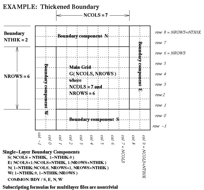
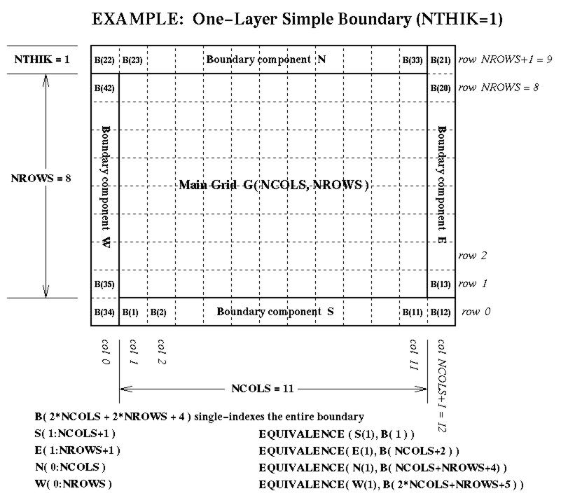
REAL*4 ARRAY( NCOLS, NROWS, NLAYS, NVARS )BNDARY3= 2:- boundary data for an external perimeter to a grid. This perimeter is
NTHIKcells wide (where you may use a negativeNTHIKto indicate an internal perimeter such as is used by ROM and RADM). The boundary array is dimensioned as follows in terms of the dimensionsNCOLSandNROWSfor the array it surrounds:...(SIZE = ABS( NTHIK )*(2*NCOLS + 2*NROWS +4*NTHIK) REAL*4 ARRAY( SIZE, NLAYS, NVARS )There are accompanying diagrams illustrating the data layout for various cases ofNTHIK:
- the general thickened-boundary case, NTHIK > 1, available as Postscript, as X11 Bitmap, as JPEG, or as GIF;
- the simple case, NTHIK = 1, available as Postscript, as X11 Bitmap, as JPEG, or as GIF;
- the internal-boundary case, NTHIK = -1 (< 0), available as Postscript, as X11 Bitmap, as JPEG, or as GIF.
IDDATA3= 3:- ID-referenced data, used to store lists of data like surface meteorology observations, pollution-monitor observations, or county-averaged concentrations. (ROM people note: this is a generalization of ROM Type 2 and 3 files, except that if you want the positions and elevations, you have to list them as variables yourself). An example of observational data with up to 100 sites, each measuring temperature, pressure, and relative humidity (in addition to having an X-Y position) is the following:
    ...
    INTEGER*4   MAXID              !  max permitted # of sites
    PARAMETER ( MAXID = 100 )
    ...
    INTEGER*4   NUMIDS             !  number of actual sites
    INTEGER*4   IDLIST( MAXID )    !  list of site ID's
    REAL*4      XLON  ( MAXID )    !  first variable in file
    REAL*4      YLAT  ( MAXID )    !  second variable
    REAL*4      TK    ( MAXID )    !  third variable
    REAL*4      PRES  ( MAXID )    !  fourth variable
    REAL*4      RH    ( MAXID )    !  fifth (last) variable
    COMMON /FOO/ NUMIDS, IDLIST, XLON, YLAT, TK, PRES, RH
NVARS3D is 5. The dimensionMAXIDmaps into theNROWS3Ddimension in the file description data structureFDESC3.EXT,for use by OPEN3() or DESC3(). To read or write this data, put the first element,NUMIDS,of this common in thearrayspot of READ3(), WRITE3(), etc.:IF ( .NOT. WRITE3( 'myfile', 'ALL', JDATE, JTIME, NUMIDS ) ) THEN ...(some kind of error happened--deal with it here) END IFPROFIL3= 4:- vertical profile data (rawindsonde data), which has a sufficiently different structure from other observational data (having possibly a site-dependent number of levels at each site) that it deserves a special data type of its own. (This is much like ROM Type 1 files.) An example of the sort of data structure needed for a rawinsonde file with NVARS3D = 3 variables
ELEV, TA,andQVgiven at up to 50 stations, each of which may have up to 100 observation levels, is given by the following. Note thatELEV= "height of the level above ground" is user-specified as one of the variables rather than supplied by the system as for ROM Type 1 files.... INTEGER*4 MXIDP ! max # of sites INTEGER*4 MXLVL ! max # of levels PARAMETER ( MAXID = 50, MXLVL = 100 ) ... INTEGER*4 NPROF ! # of actual sites INTEGER*4 PLIST( MXIDP ) ! list of site ID's INTEGER*4 NLVLS( MXIDP ) ! # of actual levels at site REAL*8 X ( MXIDP ) ! array of site X-locations REAL*8 Y ( MXIDP ) ! array of site Y-locations REAL*8 Z ( MXIDP ) ! array of site Z-locations REAL*4 ELEV ( MXLVL, MXIDP ) ! height of lvl a.g.l. REAL*4 TA ( MXLVL, MXIDP ) ! variable "TA" REAL*4 QV ( MXLVL, MXIDP ) ! variable "QV" COMMON /BAR/ NPROF, PLIST, NLVLS, X, Y, Z, ELEV, TA, QV ...The site dimensionMXIDPmaps into theNROWS3Ddimension , and the levels dimensionMXLVLmaps into theNCOLS3Ddimension in the file description (FDESC3) data structures. To read or write this data, put the first element,NPROF,of the common BAR in thearrayspot of READ3(), WRITE3(), etc.:IF ( .NOT. WRITE3( 'myfile', 'ALL', JDATE, JTIME, NPROF ) ) THEN ...(some kind of error happened--deal with it here) END IFGRNEST3= 5:- currently unused
nested-grid data should be considered as a preliminary and experimental implementation for storing multiple grids, which need not in fact have any particular relationship with each other beyond using the same coordinate system. An example of the sort of data structure needed for a nest of grids for the NVARS3D = 2 variables NO2 and O3 is the following:... INTEGER*4 MXNEST ! max # of nests INTEGER*4 MXGRID ! max # of cells (total, all grids) INTEGER*4 MXLAYS ! max # of levels PARAMETER ( MXNEST = 10, MXGRID = 10000, MXLAYS = 25 ) ... INTEGER*4 NNEST ! # of actual nests INTEGER*4 NLIST( MXNEST ) ! list of nest ID's INTEGER*4 NCOLS( MXNEST ) ! # of actual cols of nest INTEGER*4 NROWS( MXNEST ) ! # of actual rows of nest INTEGER*4 NLAYS( MXNEST ) ! # of actual lays of nest REAL*8 XN ( MXNEST ) ! array of nest X-locations REAL*8 YN ( MXNEST ) ! array of nest Y-locations REAL*8 DX ( MXNEST ) ! array of nest cell-size DX's REAL*8 DY ( MXNEST ) ! array of nest cell-size DY's REAL*4 NO2 ( MXGRID, MXLAYS, MXNEST ) ! variable "NO2" REAL*4 O3 ( MXGRID, MXLAYS, MXNEST ) ! variable "O3" COMMON /QUX/ NNEST, NLIST, NCOLS, NROWS, NLAYS, & XN, YN, DX, DY, NO2, O3 ...The nest dimensionMXNESTmaps into theNROWS3Ddimension, the cells dimensionMXGRIDmaps ontoNCOLS3D,and the layers dimensionMXLAYSmaps ontoNLAYS3Din the file description (FDESC3) data structures. To read or write this data, put the first element,NNEST,of this commonQUXin theARRAYspot of READ3(), WRITE3(), etc.:IF ( .NOT. WRITE3( 'nfile', 'ALL', JDATE, JTIME, NNEST ) ) THEN ...(some kind of error happened--deal with it here) END IFSMATRX3= 6:- sparse matrix data, which uses a "skyline-transpose" representation for sparse matrices, such as those found in the emissions model prototype. An example of the sort of data structure needed for these sparse matrices is the following:
    ...
    INTEGER     NASRC   !  total # of active cols (added over all rows)
    INTEGER     NGRID   !  number of rows in the matrix
    PARAMETER ( NASRC = 39978, NGRID = 5400 )
    ...
    INTEGER     NS( NGRID )     !  # of actual cols per row
    INTEGER     IS( NACEL )     !  column pointers
    REAL        CS( NACEL )     !  col-coefficients

    COMMON  / GRIDMAT / NS, IS, CS
In this case,NVARS3D = 1andNLAYS3D = 1. In the case ofNVARS3D > 1, multiple coefficient matrices would share the sameNSandISarrays, and similarly ifNLAYS3D > 1. The active-columns dimensionNASRCmaps into theNCOLS3Ddimension and the matrix-rows dimensionNGRIDmaps into theNROWS3Ddimension in the file description (FDESC3) data structures. To read or write this data, put the first element,NSof the commonGRIDMATin thearrayspot ofREAD3(), WRITE3(),etc., as below.IF ( .NOT. WRITE3( 'mfile', 'ALL', JDATE, JTIME, NS ) ) THEN ...(some kind of error happened--deal with it here) END IFAlternatively, "over-dimension"NSand use Fortran-77 style calls to referenceISandCS:... INTEGER NS( NGRID + 2*NACELL*NGRID ) ... CALL BLDMTX( NGRID, NASRC, NS, NS(NGRID+1), NS(NGRID+NACEL+1) ) ... IF ( .NOT. WRITE3( 'mfile', 'ALL', JDATE, JTIME, NS ) ) THEN ...(some kind of error happened--deal with it here) END IFwhereSUBROUTINE BLDMTX( NGRID, NASRC, NS, IS, CS ) INTEGER, INTENT(IN ) :: NGRID, NASRC INTEGER, INTENT( OUT) :: NS( NGRID ) INTEGER, INTENT( OUT) :: IS( NASRC ) !! in caller: NS(NGRID+1:NGRID+NACEL) REAL , INTENT( OUT) :: CS( NASRC ) !! in caller: NS(NGRID+NACEL+1: ) ...For I/O API-3.2 and later, see routines INITMTXATT(), SETMTXATT(), GETMTXATT(), CHKMTXATT(), which may be used to store, retrieve, and perform consistency-checks on extra file-header metadata for the input and output grid descriptions for matrix files.
In order for the I/O API to start itself up correctly, and in order to make sure that files are closed (and that file headers are updated) correctly, you need to call theINIT3()function at the start of your program, and theSHUT3()function (which flushes headers for, and closes all files currently open) at the end, or else theCLOSE3()function for each file opened. It is a modeling-system requirement that you should use the utility routineM3EXIT()for program termination. It will callSHUT3()correctly (as well as writing explanatory messages to the log), and then return the program's success/failure status (0 for success, non-zero for failure) to the operating system.
INIT3()is an integer function for initializing the I/O API, and must be called before any other I/O API operation. It returns the unit number to be used for the program's log (if yousetenv LOGFILE <path>, the I/O API's log and error messages will be written to this unit; otherwise, they go to standard output, unit 6).INIT3()can be called as many times as you want, to get the unit number for the program log.
SHUT3()is a logical function that returnsTRUEif the system successfully flushed all I/O API files to disk and shut itself down, andFALSEif it failed. If it failed, there probably was a hardware problem -- not much you can do about it, but at least you ought to be able to know. It is legal to callSHUT3()and close down all files currently open, and then to callINIT3()again and open new ones.
M3EXIT()is the routine used for normal program-termination. It callsSHUT3()as the final step of its operation, after writing a user supplied message with the current simulation date-and-time to the program log, and then returns the program's exit status (0 for normal completion, non-zero for program-failure) to the operating system.
CLOSE3()is a logical function that returns TRUE if the system successfully flushed the indicated file to disk and closed it, and FALSE if it failed. It should not be used by modeling programs, because its use destroys modularity; it was intended for use only by long-running visualization programs.
UseOPEN3(FNAME,FSTATUS,PGNAME)to open files, whether files that already exist or files that are new.OPEN3()is a logical function that returnTRUEwhen it succeeds, andFALSEwhen it fails. It also maintains much audit trail information stored in the file header automatically, and automates various logging activities. A couple of additional pieces of audit trail information requires a bit of work from you in setting up standard environment variables, if you want to take advantage of it: if you define the description of your program run in a text file of up to 60 lines of up to 80 characters each, and then setenv SCENFILE to that file before you run the program, thenOPEN3()will copy the SCENFILE information into theUPDSC3Dfield in the headers of any output files for that program. Also, if you setenv EXECUTION_ID to your own identifier (up to 80-character quoted line) for the program execution, it will automate the storage and the logging of that identifier in theEXECN3Dfield . Finally, if you setenv IOAPI_CHECK_HEADERS YES, then the I/O API will perform a sanity check on internal file descriptions -- checking that grid description parameters are in range, for example, or that vertical levels are either systematically increasing or systematically decreasing.The arguments to
OPEN3()are the logical nameFNAMEof the file, anINTEGER"magic number"FSTATUSindicating the type of open operation and the caller's namePGNAMEfor logging and audit-trail purposes. You can callOPEN3()many times for the same file without hurting anything, if you want -- as long as you don't first open it read-only and then try to change your mind and then open it for output, or try to open it as aNEWfile after it is already open. Names and values for the mode-of-opening magic number argument are defined in PARMS3.EXT as the following:In the last three cases, "new" "unknown" and "create/truncate," you fill in the file description from the
FSREAD3= 1 for READ-ONLY access to an existing file
This is the mode that should be used for input files.
FSRDWR3= 2 for READ/WRITE/UPDATE access to an existing file
rarely used
FSNEW3= 3 for READ/WRITE access to create a new file (file must not yet exist)
should be rarely used; leads to obscure "why is my program failing?" errors
FSUNK3= 4 for READ/WRITE/UPDATE access to a file whose existence is unknown (creates the file if it does not yet exist, otherwise, performs consistency checks with the user-supplied file definition).
This is the mode that should normally be used for output files.
FSCREA3= 5 for CREATE/TRUNCATE/READ/WRITE access to files: If the file is open, close it. If the file exists, delete it. Then create a new file according to the user-supplied file definition.
NOTE: dangerous, but the Powers That BE® insisted.
Joan Novak (EPA) and Ed Bilicki (MCNC) have declared as a software standard that modeling programs may not useFSCREA3as the mode for opening files.FSCREA3is reserved for use by analysis/data extraction programs only.
INCLUDEfile FDESC3.EXT to define the structure for the file, and then callOPEN3(). If the file doesn't exist in either of these cases,OPEN3()will use the information to create a new file according to your specifications, and open it for read/write access. In the "unknown"case, if the file already exists,OPEN3()will perform a consistency check between your supplied file description and the description found in the file's own header, and will returnTRUE(and leave the file open) only if the two are consistent. Sample calls toOPEN3()for an input file 'myfile' and an output file 'my_newfile' might look like the following:... IF ( .NOT OPEN3( 'myfile', FSREAD3, 'my program') ) THEN ...(some kind of error happened--deal with it here) END IF ... ... (First, fill in the file's description for 'my_newfile' here. ... Then open it:) IF ( .NOT. OPEN3( 'my_newfile', FSNEW3, 'my program' ) ) THEN ...(some kind of error happened--deal with it here) END IFThere are also several sample programs that demonstrate how to use the I/O API to create various kinds of files -- gridded, boundary, and ID-referenced, with one or multiple layers, and either time-stepped or time-independent.To get a file's description, you use the
DESC3(FNAME)function. When you callDESC3(), it puts the file's complete description in the standard file description data structures in FDESC3.EXT. Note that the file must have been opened prior to callingDESC3(). A typical output-file call sequence might look like:... IF ( .NOT. OPEN3( 'myfile', FSUNKN3, 'myprogram' ) ) THEN ...(some kind of error happened--deal with it here) ELSE IF ( .NOT. DESC3( ' myfile' ) ) THEN ...(some kind of error happened--deal with it here) ELSE ...(the FDESC3 commons now contain the file description: ... data type, dimensions, starting date&time, timestep, ... list of variables and their descriptions, etc.) END IF ...
There are four routines with varying kinds of selectivity used to read or otherwise retrieve data from files:READ3(),XTRACT3(),INTERP3(), andDDTVAR3(). All of them are logical functions that returnTRUEwhen they succeed,FALSEwhen they fail.The first two require that the time step you request be on the file -- they won't give you data for the half-hour, for example, if the file has hourly data only. Because it optimizes the interpolation problem for you,
READ3(FNAME,VNAME,LAYER,JDATE,JTIME,BUFFER)- reads one variable
VNAMEor all variables (ifVNAME=ALLVARS3='ALL') and one or all layers (ifLAYER=ALLAYSS3=-1) from the fileFNAMEfor a particular date and timeJDATE:JTIME;
XTRACT3(FNAME,VNAME,LAY0,LAY1,ROW0,ROW1,COL0,COL1,JDATE,JTIME,BUFFER)- reads a windowed subgrid
BUFFER=GRID(COL0:COL1,ROW0:ROW1,LAY0:LAY1)whereFNAMEmust be of typeGRDDED3, with full-grid array dimensionsGRID(NCOLS3D,NROWS3D,NLAYS3D). Otherwise, it is much likeREAD3();
INTERP3(FNAME,VNAME,CALLER,JDATE,JTIME,RSIZE,BUFFER)- time-interpolates the requested variable from the requested file to the requested date and time (optimizing disk accesses and interpolation-buffer manipulation internally behind the scenes).
FNAMEmust have typeGRDDED3, CUSTOM3,orBNDARY3, andRSIZE=NCOLS3D*NROWS3D*NLAYS3Dmust be the total array-size.
DDTVAR3(FNAME,VNAME,CALLER,JDATE,JTIME,RSIZE,BUFFER)- computes the time-derivative, much as
INTERP3()time-interpolates.
INTERP3()is probably the most useful of these routines. Note that it has asizeargument -- you tell it how much data you expect, and it checks that against how much data the file thinks you ought to get, for error checking purposes. A typicalINTERP3()call to read/interpolate the variableHNO3to 12:37 PM on February 4, 1987 (Models-3 Convention date&time 1987035:123000) might look like:... CHARACTER*16 FNAME, VNAME REAL*4 ARRAY( NCOLS, NROWS, NLAYS ) ... IF ( .NOT. INTERP3( 'myfile', 'HNO3', 1987035, 123700, & NCOLS*NROWS*NLAYS, ARRAY ) ) THEN ...(some kind of error happened--deal with it here) END IFWithREAD3()andXTRACT3(), you can use the "magic values"ALLVAR3'(= 'ALL', defined in PARMS3.EXT) orALLAYS3(= -1, also defined in PARMS3.EXT) as variable name and/or layer number to read all variables or all layers from the file, respectively.For time independent files, the date and time arguments are ignored.
You use the logical functionWRITE3(FNAME,VNAME,JDATE,JTIME,BUFFER)to write data to files. For gridded, boundary, and custom files, you may write either one time step of one variable at a time, or one entire time step of data at a time (in which case, use "magic value"ALLVAR3(='ALL', defined inPARMS3.EXT) as the variable-name). For ID-referenced, profile, and grid-nest files, you must write an entire time step at a time (i.e., the variable-name must beALLVAR3).WRITE3()is affected by standard environment variable IOAPI_LOG_WRITE (which has default value "YES"); normallyWRITE3()generates a log message for each write-operation successfully completed. However, if yousetenv IOAPI_LOG_WRITE NOthen these messages will be suppressed. TypicalWRITE3()calls to write data for date and timeJDATE:JTIMEmight look like the following:... REAL*4 ARRAYA( NCOLS, NROWS, NLAYS ) REAL*4 ARRAYB( NCOLS, NROWS, NLAYS, NVARS ) ... IF ( .NOT. WRITE3( 'myfile', 'HNO3', JDATE, JTIME, ARRAYA ) ) THEN ...(some kind of error happened--deal with it here) END IF IF ( .NOT. WRITE3( 'afile', 'ALL', JDATE, JTIME, ARRAYB ) ) THEN ...(some kind of error happened--deal with it here) END IF
Throughout the EDSS and Models-3 systems -- and particularly in the I/O API -- dates and times (and time-steps) are stored as integers, using the coding formatsHHMMSS = 10000 * hour + 100 * minutes + seconds YYYYDDD = 1000 * year + daywhere the year is 4-digits (1994, say, rather than just 94), and the day is the Julian day-number (1,...,365 or 366). By convention, dates and times are stored in Greenwich Mean Time.There are a number of utility routines for date and time manipulation, , as well as a number of programs for date and time manipulation; some of these programs are designed for interactive use, others for scripting. The most frequently used of these programs are juldate, for converting calendar dates to Julian dates, and gregdate, for converting Julian dates to calendar dates and reporting the day-of-the-week. Both of these programs also report whether daylight savings time is in effect for the specified date.
The most frequently used utility routines for manipulating dates and times are described below. Note that for these routines, time steps may perfectly well be negative -- just make sure you keep the parts all positive or all negative; a time step of -33000 means to step three and a half hours into the past, for example. This way of representing dates and times is easy to understand and manipulate when you are watching code in the debugger (you don't have to turn "seconds since Jan. 1, 1970" into something meaningful for your model run, nor do you have to remember whether April has 30 days or 31 when your model run crosses over from April to May). Some useful utility routines for manipulating dates and times are the following:
NEXTIME( JDATE, JTIME, TSTEP )is a subroutine which updates date and timeJDATE:JTIMEby the time stepTSTEP(which may be either positive or negative);
LASTTIME( SDATE,STIME,TSTEP,NRECS, EDATE,ETIME )is a subroutine which computes the ending date&timeEDATE:ETIMEfor a time step sequence starting atSDATE:STIME, with time stepTSTEPandNRECSsteps.
Safe fromINTEGERoverflow, even for multiple centuries;
TIME2SEC( TSTEP )is an integer function which returns the number of seconds in the time intervalTSTEP;
SEC2TIME( SECS )is an integer function which returns the time intervalHHMMSSfor the specified number of seconds;
SECSDIFF( ADATE, ATIME, ZDATE, ZTIME )is an integer function which returns the number of seconds fromADATE:ATIMEtoZDATE:ZTIME;
Subject toINTEGERoverflow for periods longer than aboaut 21 years.
DT2STR( JDATE, JTIME )is aCHARACTER*24utility function which returns a string for the date and time, as for example "09:12:25 April 28, 1994"
CURREC( JDATE, JTIME, SDATE, STIME, TSTEP,
              CDATE, CTIME )
is anINTEGERfunction which returns the record number for the time step that containsJDATE:JTIMEin the time step sequenceSDATE:STIME:TSTEP, even ifJDATE:JTIMEis not an exact time step, and setsCDATE:CTIMEto the exact date&time for this time step sequence. IfJDATE:JTIMEis beforeSDATE:STIME, returns -1.
HHMMSS( JTIME )is aCHARACTER*10utility function which returns the string for the time "HH:MM:SS" (like the first field fromDT2STR());
ISDSTIME( JDATE )is aLOGICALutility function which returnsTRUEwhen daylight savings time is effect forJDATE
JSTEP3( JDATE, JTIME, SDATE, STIME, TSTEP )is anINTEGERfunction which returns the timestep-record number corresponding toJDATE:JTIMEifJDATE:JTIMEis exactly on the timestep sequence, or -1 otherwise.
MMDDYY( JDATE )is aCHARACTER*14utility function which returns a string "Month DD, YYYY" for the date (like the second field fromDT2STR());
DAYMON( JDATE, MONTH, MDAY )is a utility subroutine which returns the month (1, ..., 12) and day of month (1, ..., 31) for the specified Julian date;
WKDAY( JDATE )is a utility integer function which returns the day-of-week (1=Monday, ..., 7=Sunday) for the specified Julian date;
NOTE: Non-standard week (beginning with Monday instead of Sunday) dictated by the emissions modelers.
JULIAN( YYYY, MONTH, MDAY )is a utility integer function which returns the Julian day (1, ..., 365,366) for a specified year, month (1-12), and day of month (1-31).
Horizontal coordinate systems (or "map projections") define CartesianX-Ycoordinate systems on regions on the surface of the Earth. Typically, they have various defining parameters, which are given in term of the fundamental "Lat-Lon" or "geographic" coordinate system. See https://en.wikipedia.org/wiki/ISO_6709 for a description of the international standard ISO 6709 for representation of latitude, longitude and altitude for geographic point locations.For example, a Lambert coordinate system is the result of projecting the surface of the Earth from the center of the Earth onto a cone with axis the North-South axis of the Earth, that intersects the Earth at two latitudes ALPHA and BETA, cutting it diametrically opposite a central longitude GAMMA and unrolling it flat, then placing the coordinate origin (X=0,Y=0 at longitude and latitude XCENT,YCENT.
Horizontal Grids are then defined in terms of horizontal coordinate systems. In particular, regular grids have rectangular sides parallel to the coordinate axis, a starting corner XORIG,YORIG defined in term of the map-projection coordinates, a constant cell size XCELL,YCELL, and dimensions NCOLS in the X direction and NROWS in the Y direction, so that the cell at column and row C,R is defined by inequalities
XORIG + (C-1)*XCELL ≤ X ≤ XORIG + C*XCELLNote that in principle either of XCELL,YCELL may be positive or negative. It is usual for both to be positive for meteorological and air quality modeling; however, be aware that much GIS related data has positive XCELL and negative YCELL (so-called "scan-line order")
YORIG + (R-1)*XCELL ≤ Y ≤ YORIG + R*YCELL
Grid Boundary data structures are defined by a thickness NTHIK cells around the perimeter of a rectangular grid.
Vertical coordinate systems typically have some sort of meteorologically-defined vertical coordinate variable; vertical grids are rarely regular, and instead have a dimensions NLAYS and cells with non-uniform thicknesses V(0), V(1), ..., V(NLAYS), where V is the vertical coordinate variable. Then cells are defined by "layer-surface" inequalities, e.g. for layer L,
V(L-1) ≤ V ≤ V(L)Frequently, the vertical coordinate-variable increases with altitude; however, be aware that in some cases (for instance, the MM5 meteorological model), the opposite is true.See this page for a more-complete description of I/O API map-projection and grid-description conventions.
There are a number of utility routines for grid and coordinate related tasks (such as coordinate-transforms and interpolation), which are indexed here. In particular, see
MODULE MODGCTP, which provides a number of routines that use the USGS Grid Coordinate Transformation Package (GCTP) routines.A number of the m3tools programs are designed for grid- and coordinate-related tasks. Particularly notable are the following:
m3wndwandbcwndw: extract data data from a gridded file to a subgrid window or its boundary.
m3cple: copy to the same grid, or interpolate to another grid a time sequence of all variables from a source file to a target file, under the optional control of a "synch file".
mtxcalcandmtxcple: build a grid-to-grid sparse-matrix transform file using a sub-sampling algorithm, and use it to re-grid a time sequence of all variables from a source file to a target file, respectively.
projtool: Perform coordinate conversions and grid-related computations,
latlon: construct GRIDDED and/or BOUNDARY files with variables the cell-centerLATandLON.
gridprobe: Extract ASCII and/or I/O API time series from aGRIDDEDfile for a set of Lat-Lon designated points.
- MODULE MODGCTP provides parameters and routines for map-transform operations and interpolation, using USGS coordinate transform package GCTP.
- MODULE MODNCFIO provides parameters and function-declarations for netCDF, and for PnetCDF, if PnetCDF/MPI distributed-I/O is enabled.
Can be used to replaceINCLUDE-file NETCDF.EXT or netcdf.inc, Also includes new high-level routines for inquiring about, reading, and writing variables from "raw" netCDF files.
- MODULE MODWRFIO provides high level I/O routines for opening, creating, reading, and writing WRF-format-netCDF files.
- MODULE MODMPASFIO provides high level MPAS-format-netCDF I/O routines, together with unstructured-MPAS-grid description for MPAS domains, related parameters and state variables, and various MPAS-grid geometry and utility routines
- There are utility routines for a wide variety of modeling related tasks, including retrieval of environment variables, prompting the user for values of various kinds, searching and sorting data, various text transformations, and opening "ordinary" files.
- There are utility programs for a variety of analysis and data manipulation tasks. Source code for all of these programs is available for you to examine and use as part of the I/O API download; certain of these are annotated and available for you to view in web form.
Here is an example of the typical outline for a program that processes time stepped data (i.e., most modeling programs, and most analysis programs), using the most-common I/O API routines:PROGRAM MYPROGRAM ... USE M3UTILIO IMPLICIT NONE ... CHARACTER*16, PARAMETER :: PNAME = 'MYPROGRAM' CHARACTER*72, PARAMETER :: BAR = & '-=-=-=-=-=-=-=-=-=-=-=-=-=-=-=-=-=-=-=-=-=-=-=-=-=-=-=-=-=-=-=-=-=-=-=-' ... INTEGER LUNIT ! unit number for log file INTEGER ISTAT INTEGER SDATE, STIME, TSTEP, NRECS INTEGER JDATE, JTIME, N REAL BARFAC ! used in computing BAR INTEGER NCOLS ! number of grid columns INTEGER NROWS ! number of grid rows INTEGER NLAYS ! number of layers INTEGER NTHIK ! bdy thickness INTEGER NVARS ! number of variables INTEGER GDTYP ! grid type: 1=LAT-LON, 2=Lambert, ... INTEGER VGTYP ! vertical coord type REAL*8 P_ALP ! first, second, third map REAL*8 P_BET ! projection descriptive REAL*8 P_GAM ! parameters. REAL*8 XCENT ! lon for coord-system X=0 REAL*8 YCENT ! lat for coord-system Y=0 REAL*8 XORIG ! X-coordinate origin of grid (map units) REAL*8 YORIG ! Y-coordinate origin of grid REAL*8 XCELL ! X-coordinate cell dimension REAL*8 YCELL ! Y-coordinate cell dimension REAL VGTOP ! vertical coord top (for sigma coords) REAL VGLEV( MXLAYS3+1 ) ! "full" levels ... CHARACTER*256 MESG ... REAL, ALLOCATABLE :: QV( :,:,: ) REAL, ALLOCATABLE :: TA2( :,: ) REAL, ALLOCATABLE :: BAR( :,: ) ... !!............. begin body of program ....................... LUNIT = INIT3() WRITE( LUNIT, '( 5X, A )' ) ' ',BAR, ' ', & 'Program MYPROGRAM to compute BAR using data from files METCRO2D and', & 'METCRO3D, and write the result to file OUTCRO2D.', & '', & 'THE PROGRAM WILL PROMPT YOU for the starting and ending date&time, and', & 'time step to process, and the factor BARFAC to use in the computation.', & '', & 'PRECONDITIONS REQUIRED:', & ' setenv METCRO2D <path name>', & ' setenv METCRO3D <path name>', & ' setenv OUTCRO2D <path name for output file>', & BAR, '' ... !!........ Open input files. Perform consistency checks. IF ( .NOT.OPEN3( 'METCRO3D', FSREAD3, PNAME ) ) THEN CALL M3EXIT( PNAME, 0,0, 'Could not OPEN3(METCRO3D,...)', 2 ) ELSE IF ( .NOT.DESC3( 'METCRO3D' ) ) THEN CALL M3EXIT( PNAME, 0,0, 'Could not DESC3(METCRO3D)', 2 ) ELSE NCOLS = NCOLS3D NROWS = NROWS3D NLAYS = NLAYS3D GDTYP = GDTYP3D P_ALP = P_ALP3D P_BET = P_BET3D P_GAM = P_GAM3D XCENT = XCENT3D YCENT = YCENT3D XORIG = XORIG3D YORIG = YORIG3D XCELL = XCELL3D YCELL = YCELL3D VGTYP = VGTYP3D VGTOP = VGTOP3D VGLEV( : ) = VGLVS3D( : ) END IF IF ( .NOT.OPEN3( 'METCRO2D', FSREAD3, PNAME ) ) THEN CALL M3EXIT( PNAME, 0,0, 'Could not OPEN3(METCRO2D,...)', 2 ) ELSE IF ( .NOT.DESC3( 'METCRO2D' ) ) THEN CALL M3EXIT( PNAME, 0,0, 'Could not DESC3(METCRO2D)', 2 ) ELSE IF ( .NOT.FILCHK3( 'METCRO2D', GRDDED3,NCOLS, NROWS, 1, 1 ) ) THEN CALL M3EXIT( PNAME, 0,0, 'Inconsistent dimensions for "METCRO2D"', 2 ) ELSE IF ( .NOT.GRDCHK3( 'METCRO2D', & P_ALP, P_BET, P_GAM, XCENT, YCENT, & XORIG, YORIG, XCELL, YCELL, & 1, VGTYP, VGTOP, VGLEV ) ) THEN CALL M3EXIT( PNAME, 0,0, 'Inconsistent map-projection or grid for "METCRO2D"', 2 ) END IF ... !!........ Get SDATE, STIME, TSTEP, NRECS, BARFAC from the user: CALL RUNSPEC( METFILE, .FALSE., SDATE, STIME, TSTEP, NRECS ) BARFAC = GETVAL( 0.0, 1.0, 0.7071, 'Enter BARFAC' ) ... !!........ Open output file(s). First, fill in FDESC... !!........ (borrowing parts of the FDESC from METCRO2D) ... NVARS3D = ... NLAYS3D = 1 SDATE3D = SDATE STIME3D = STIME TSTEP3D = TSTEP ... VNAME3D(1) = 'BAR' VTYPE3D(1) = M3REAL UNITS3D(1) = 'Somethings' VDESC3D(1) = 'dingbat that plings the inghams' ... IF ( .NOT.OPEN3( 'OUTCRO2D', FSUNKN3, PNAME ) ) THEN CALL M3EXIT( PNAME, 0,0, 'Could not OPEN3(OUTCRO2D,...)', 2 ) END IF ... !!........ Allocate arrays ALLOCATE ( TA2( NCOLS,NROWS ), & BAR( NCOLS,NROWS ), & QV( NCOLS,NROWS,NLAYS ), STAT = ISTAT IF ( ISTAT .NE. 0 ) THEN WRITE( MESG, '(A, I9)' ) 'Allocation failure: STAT=', ISTAT CALL M3EXIT( PNAME, 0,0, MESG, 2 ) END IF ... !!........ Main processing loop JDATE = SDATE JTIME = STIME DO N = 1, NRECS !! loop on timesteps WRITE( MESG, '(A,I9.7,A,I6.6)' ) 'Processing date and time', JDATE, ':', JTIME CALL M3MESG( MESG ) ... IF ( .NOT.READ3( 'METCRO2D', 'TA2', JDATE, JTIME, 1, TA2 ) ) THEN MESG = 'ERROR reading "TA2" from "METCRO2D"' CALL M3EXIT( PNAME, 0,0, MESG, 2 ) END IF IF ( .NOT.READ3( 'METCRO3D', 'QV', JDATE, JTIME, ALLAYS3, QV ) ) THEN MESG = 'ERROR reading "QV" from "METCRO3D"' CALL M3EXIT( PNAME, 0,0, MESG, 2 ) END IF ... [compute BAR from TA2,QV etc... using BARFAC, etc.] ... IF ( .NOT.WRITE3( 'OUTCRO2D', 'BAR', JDATE, JTIME, BAR ) ) THEN MESG = 'ERROR writing "BAR" to "OUTCRO2D"' CALL M3EXIT( PNAME, 0,0, MESG, 2 ) END IF ... CALL NEXTIME( JDATE, JTIME, TSTEP ) END DO !! end loop on timesteps ... CALL M3EXIT( PNAME, 0, 0, 'Successful completion', 0 ) END PROGRAM FOO
Next: Changes from the Previous I/O API Version
To: Models-3/EDSS I/O API: The Help Pages
$Id: TUTORIAL.html 239 2023-03-14 15:06:03Z coats $