In SMOKE, there are two major processing routes that you can take for area sources: the typical route and the pregridded data route. (Recall that by “area sources” in SMOKE we mean stationary area/nonpoint sources and nonroad mobile sources.)
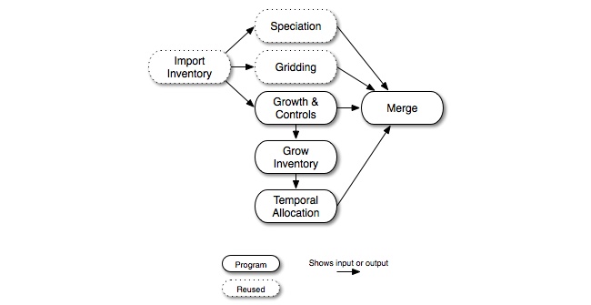
The typical route involves processing data identified by country/state/county codes and SCCs. The processing steps vary depending on whether you are doing base-case processing or future- or past-year processing. The steps for base-year processing are shown in Figure 2.8, “Base case area-source processing steps”. In Figure 2.4, “Parallel approach to emissions processing”, we also included the major intermediate vectors and matrices; please refer to that diagram for those details. The inventory import step reads the raw emissions data, screens them, processes them, and converts the raw data to the SMOKE intermediate inventory file (inventory vectors in Figure 2.4, “Parallel approach to emissions processing”). The emissions in the inventory file are subdivided to hourly emissions during temporal allocation; assigned chemical speciation factors during speciation, and assigned spatial allocation factors during gridding. The merge step combines the hourly emissions, speciation matrix, and gridding matrix to create model-ready emissions.

In Figure 2.9, “Future- or past-year growth and optional control area-processing steps”, we show the area-source processing steps for future- or past-year processing. This processing is similar to the base-year processing flow, except the growth and controls step is added to create the growth matrix and optionally one or more control matrices. The grow inventory step applies the growth matrix to convert the base-year inventory to a future or past year. Also, the control matrix can optionally be used in the merge step to apply control factors to the future- or past-year emissions. The steps shown with dotted lines represent steps that can be reused from the base-year processing because they do not depend on any of the new steps.
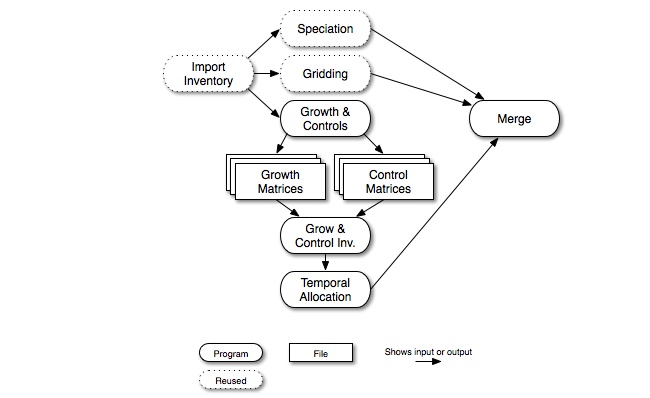
Finally, inventory controls as well as growth can be applied at the front end of processing if such a scheme is needed (Figure 2.10, “Alternative future- or past-year growth and control area-processing steps”). This method permits up to 80 growth and/or control matrices to be applied to an inventory, whereas the method shown in Figure 2.9, “Future- or past-year growth and optional control area-processing steps” allows only one control matrix in the merge step, although any number of growth matrices on the front end. The processing scheme shown in Figure 2.10, “Alternative future- or past-year growth and control area-processing steps” can therefore be useful when mixing and matching many control strategies for simulations.
In sections later in this chapter, we describe the SMOKE programs that are needed for each of these processing steps and additional details about what activities are accomplished during each step. These sections are:
The second processing approach for area sources involves using pregridded data. As indicated in Section 2.8.1, “Summary of SMOKE processing categories”, area sources can be specified by grid cell instead of by country/state/county code and SCC. This optional approach to modeling area sources requires the inventory emissions data to be gridded prior to inventory import. The gridded area sources do not have country/state/county codes or SCCs, and can be provided via an I/O API time-independent gridded data file. The flow diagrams that describe this type of processing are identical to those in Figure 2.8, “Base case area-source processing steps”, Figure 2.9, “Future- or past-year growth and optional control area-processing steps”, and Figure 2.10, “Alternative future- or past-year growth and control area-processing steps”. Although the gridding step is quite trivial when the grid cell numbers are already specified, the gridding step must still be run to create a gridding matrix required for the merge step.
The disadvantage of using pregridded emissions for area-source processing is that there are no country/state/county codes and SCCs to use in the cross-referencing of any processing step. Therefore, temporal profiles, speciation profiles, growth factors, and control factors must be applied uniformly across the model grid by pollutant.
Emissions from area sources are sometimes available as day- or hour-specific values. Smkinven can import the day- and hour-specific data, and it can also convert the hour-specific data to hour-specific temporal profiles. When these data are available, the Temporal program overrides the annual or daily emissions with the most specific data available. If day-specific data are available, Temporal uses them to overwrite the annual or average-day emissions during the time periods that these data are available. If hour-specific data are available, Temporal uses them to overwrite the annual, average-day emissions, or day-specific emissions data.