Last updated: 12/30/2015
SMOKE-MOVES is a set of methodologies and software tools to help use output from MOVES2014 as inputs to SMOKE. More information about each of these models can be found at:
MOVES stands for MOtor Vehicle Emission Simulator, and MOVES2014 is the latest version of MOVES. In the SMOKE-MOVES system, MOVES2014 is used to generate emission factors for mobile sources. MOVES2014 can generate emission factors for criteria pollutants, greenhouse gases, and air toxics. These factors are combined with activity data like vehicle miles travelled and vehicle population to estimate mobile emissions. MOVES2014 generates four types of emission factors:
Because generating emission factors is a time consuming task, it’s important to restrict the needed MOVES2014 runs as much as possible. Since the emission factors are temperature dependent, MOVES2014 can be run to only generate factors for temperatures that are in the modeling domain (geographic area and time period of interest). Gridded, hourly meteorology data is processed by the program Met4moves to determine which temperature combinations and profiles should be processed through MOVES2014.
In addition to temperature data, MOVES2014 requires county-level data describing the vehicles and roads to be modeled. This data includes:
Counties with similar county-level data can be grouped together into a reference county. MOVES2014 is run to generate a suite of emission factors for each reference county, covering the different temperatures and fuel months needed. Then, all counties assigned to that reference county will share the generated emission factors.
The runspec_generator.pl script takes a list of reference counties and the outputs produced by Met4moves, and generates the run specification files (runspecs) used by MOVES2014 along with scripts to drive MOVES2014. The runspecs created by the runspec generator script are crafted to run MOVES2014 in emission factor mode with the appropriate options to generate the suite of emission factors needed for later processing in SMOKE.
MOVES2014 is run using the outputs from the runspec generator script. The outputs from MOVES2014 are emission factors stored in a MySQL database. The script moves2smkEF.pl extracts the needed emission factors from the database and produces output that is readable by SMOKE.
The SMOKE emissions model combines county-level activity data with the emission factors created by MOVES2014 to produce mobile emission estimates. Three different types of activity data are input to SMOKE as inventories:
The activity data are broken down by county and SCC, where the SCC encodes the fuel type, vehicle type, road type, and emissions process for each source.
SMOKE consists of several individual programs. For onroad mobile emissions, the programs used are:
Smkinven: reads the activity inventories and outputs intermediate files for further processing
Grdmat: determines how sources in the inventory should be assigned to grid cells in the modeling domain
Spcmat: handles calculating model species from emissions; MOVES2014 is capable of outputting emission factors as both pollutants (mass-based) and model species (mole-based) for the CB05 and CB6 speciation mechanisms
Temporal: transforms annual or monthly activity inventory data into hourly estimates
Movesmrg: combines the activity data with the MOVES2014 emission factors to produce estimates of onroad mobile emissions; Movesmrg can output state, county, and SCC-level emissions summaries, and hourly, gridded emissions ready for use in air quality model like CMAQ
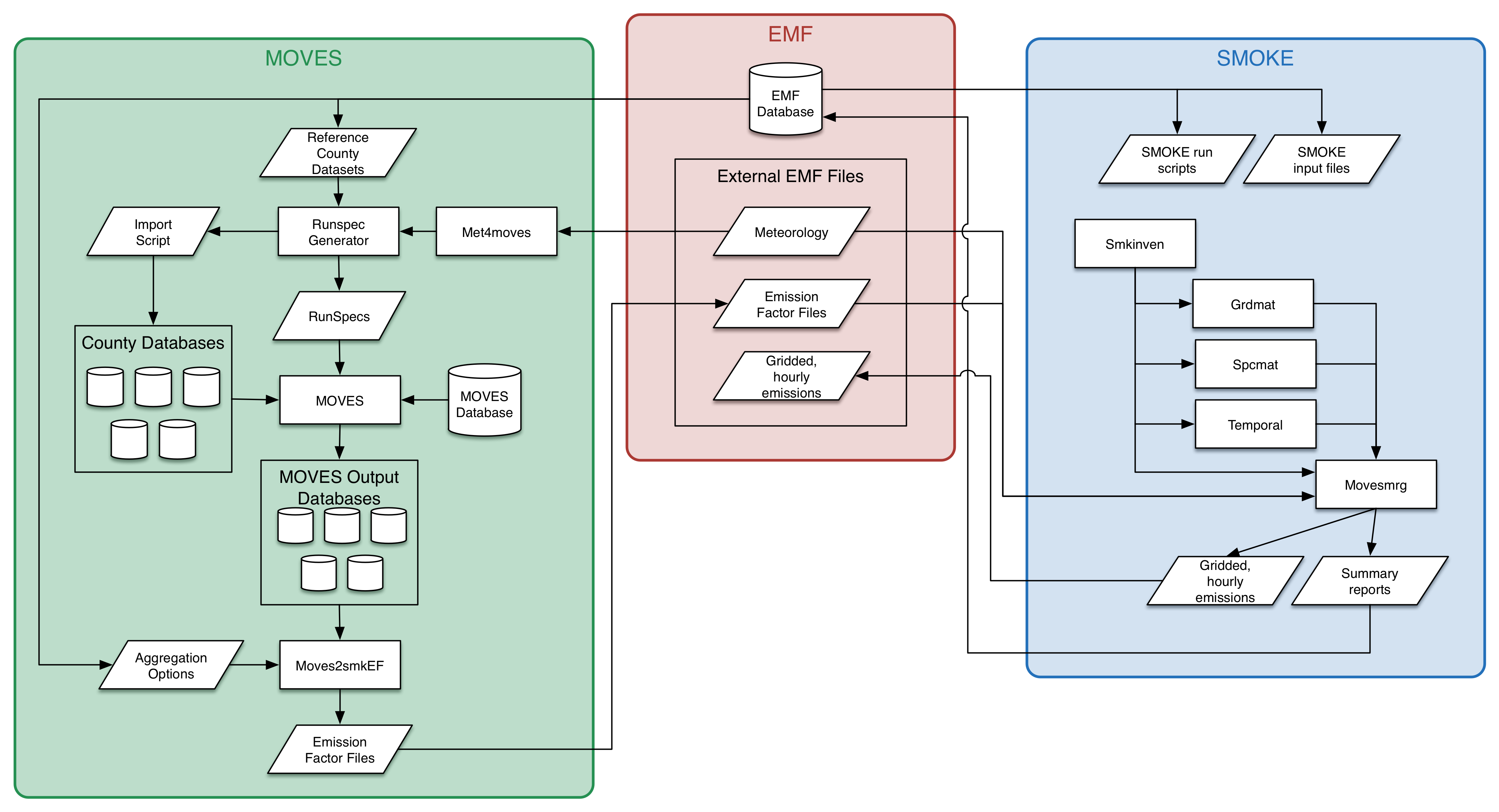
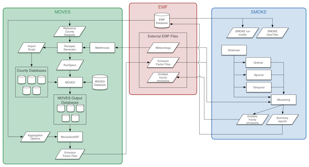
The interactions between each component of SMOKE-MOVES and the EMF are detailed in Figure 1-1. View larger.
The EMF is shown in the middle of the diagram and handles coordinating the data and workflow. The EMF database contains various datasets used by SMOKE-MOVES: activity inventories, SMOKE input files like the temporal allocation factors, and reference county data needed by MOVES2014. The EMF also manages various external datasets. These are large data files that are not imported into the EMF database, but the EMF does have metadata about each dataset. In SMOKE-MOVES, these external datasets include the gridded, hourly meteorology data files; the emission factor files; and the gridded, hourly emissions files.
In the EMF, cases are used to organize data and settings needed for model runs. For example, a case might run MOVES2014 to generate emission factors for a set of reference counties, or a case may run SMOKE to create inputs for CMAQ. Cases are a flexible concept to accommodate many different types of processing. Cases are organized into:
When a job is run, it can produce messages that are stored as the history for the job. A job may also produce data files that are automatically imported into the EMF; these datasets are referred to as outputs for the job.
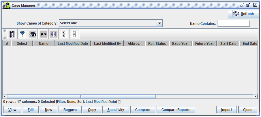
To work with cases in the EMF, select the Manage menu and then Cases. This opens the Case Manager window, which will initially be empty as shown in Figure 2-1.
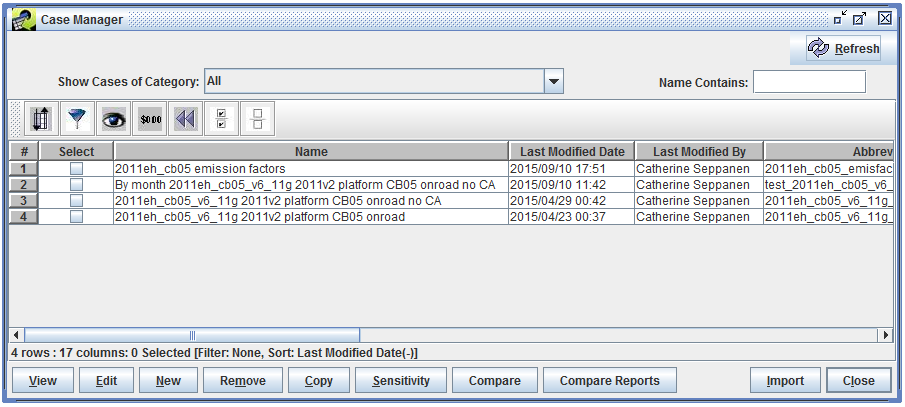
To show all cases currently in the EMF, use the Show Cases of Category pull-down to select All. The Case Manager window will then list all the cases as shown in Figure 2-2.
The Case Manager window shows a summary of each case. Table 2-1 lists each column in the window. Many of the values are optional and may or may not be used depending on the specific model and type of case.
| Column | Description |
|---|---|
| Name | The unique name for the case. |
| Last Modified Date | The most recent date and time when the case was modified. |
| Last Modified By | The user who last modified the case. |
| Abbrev. | The unique abbreviation assigned to the case. |
| Run Status | The overall run status of the case. Values are Not Started, Running, Failed, and Complete. |
| Base Year | The base year of the case. |
| Future Year | The future year of the case. |
| Start Date | The starting date and time of the case. |
| End Date | The ending date and time of the case. |
| Regions | A list of modeling regions assigned to the case. |
| Model to Run | The model that the case will run. |
| Downstream | The model that the case is creating output for. |
| Speciation | The speciation mechanism used by the case. |
| Category | The category assigned to the case. |
| Project | The project assigned to the case. |
| Is Final | Indicates if the case has been marked as final. |
In the Case Manager window, the Name Contains textbox can be used to quickly find cases by name. The search term is not case sensitive and the wildcard character * (asterisk) can be used in the search.
To work with a case, select the case by checking the checkbox in the Select column, then click the desired action button in the bottom of the window. Table 2-2 describes each button.
| Command | Description |
|---|---|
| View | Opens the Case Viewer window to view the details of the case in read-only mode. |
| Edit | Opens the Case Editor window to edit the details of the case. |
| New | Opens the Create a Case window to start creating a new case. |
| Remove | Removes the selected case; a prompt is displayed confirming the deletion. |
| Copy | Copies the selected case to a new case named “Copy of case name”. |
| Sensitivity | Opens the sensitivity tool, used to make emissions adjustments to existing SMOKE cases. |
| Compare | Generates a report listing the details of two or more cases and whether the settings match. |
| Compare Reports | Opens the Compare Case window which can be used to compare the outputs from different cases. |
| Import | Opens the Import Cases window where case information that was previously exported from the EMF can be imported from text files. |
| Close | Closes the Case Manager window. |
| Refresh | Refreshes the list of cases and information about each case. (This button is in the top right corner of the Case Manager window.) |
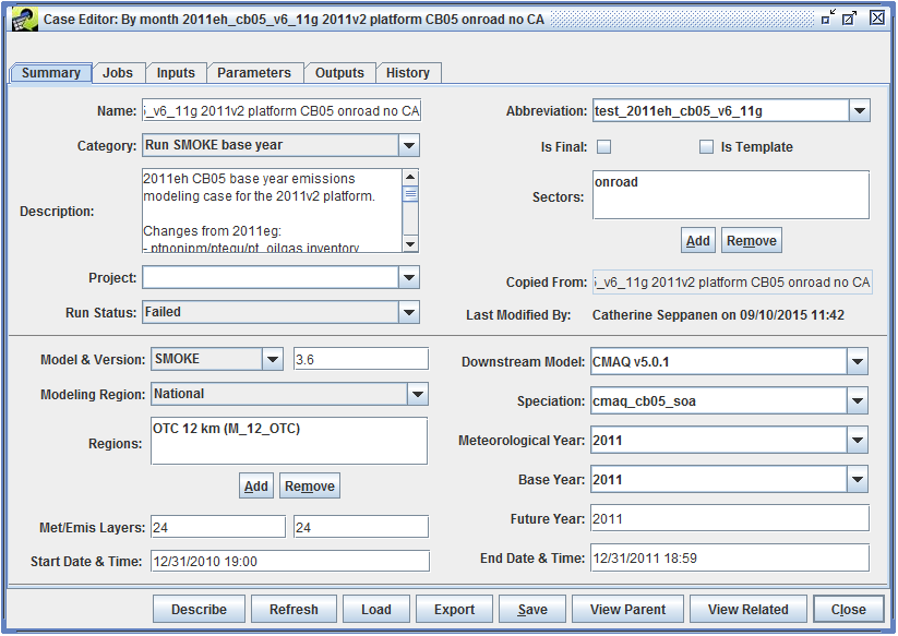
To view or edit the details of a case, select the case in the Case Manager window, then click the View or Edit button. Figure 2-3 shows the Case Viewer window, while Figure 2-4 shows the Case Editor window for the same case. Data in the Case Viewer window is not editable, and the Case Viewer window does not have a Save button.
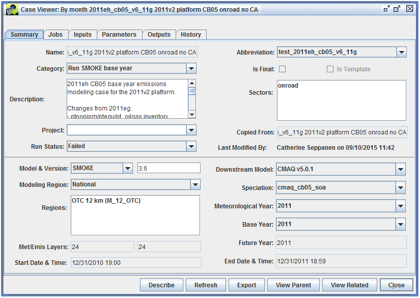
The Case Viewer and Case Editor windows split the case details into six tabs. Table 2-3 gives a brief description of each tab.
| Tab | Description |
|---|---|
| Summary | Shows an overview of the case and high-level settings |
| Jobs | Work with the individual jobs that make up the case |
| Inputs | Select datasets that will be used as inputs to the case’s jobs |
| Parameters | Configure settings and other information needed to run the jobs |
| Outputs | View and export the output datasets created by the case’s jobs |
| History | View log and status messages generated by individual jobs |
There are several buttons that appear at the bottom of the Case Viewer and Case Editor windows. The actions for each button are described in Table 2-4.
| Command | Description |
|---|---|
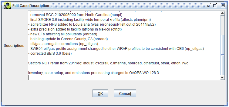
| Describe | Shows the case description in a larger window. If opened from the Case Editor window, the description can be edited (see Figure 2-5). |
| Refresh | Reload the case details from the server. |
| Load (Case Editor only) | Manually load data created by CMAQ jobs into the EMF. |
| Export | Exports the case settings to text files. See Section 2.1. |
| Save (Case Editor only) | Save the current case. |
| View Parent | If the case was copied from another case, opens the Case Viewer showing the original case. |
| View Related | View other cases that either produce inputs used by the current case, or use outputs created by the current case. |
| Close | Closes the Case Viewer or Case Editor window |
The Export button at the bottom of the Case Viewer or Case Editor window can be used to export the current case. Clicking the Export button will open the Export Case dialog shown in Figure 2-6.
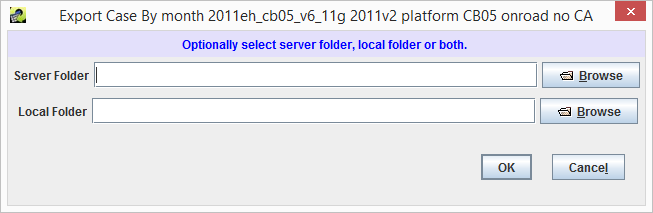
The case can be exported to text files either on the EMF server or directly to a local folder. After selecting the export location, click OK to export the case. The export process will create three text files, each named with the case’s name and abbreviation. Table 2-5 describes the contents of the three files.
| File Name | Description |
|---|---|
| case_name_abbrev_Summary_Parameters.csv | Settings from the Summary tab, and a list of parameters for the case |
| case_name_abbrev_Jobs.csv | List of jobs for the case with settings for each job |
| case_name_abbrev_Inputs.csv | List of inputs for the case including the dataset name associated with each input |
The exported case data can be loaded back into the EMF using the Import button in the Case Manager window.
Figure 2-7 shows the Summary tab in the Case Editor window.
The Summary tab shows a high-level overview of the case including the case’s name, abbreviation, and assigned category. Many of the fields on the Summary tab are listed in the Case Manager window as described in Table 2-1.
The Is Final checkbox indicates that the case should be considered final and should not have any changes made to it. The Is Template checkbox indicates that the case is meant as a template for additional cases and should not be run directly. The EMF does not enforce any restrictions on cases marked as final or templates.
The Description textbox allows a detailed description of the case to be entered. The Describe button at the bottom of the Case Editor window will open the case description in a larger window for easier editing.
The Sectors box lists the sectors that have been associated with the case. Click the Add or Remove buttons to add or remove sectors from the list.
A case can optionally be assigned to a project using the Project pull-down menu.
If the case was copied from a different case, the parent case name will be listed by the Copied From label. This value is not editable. Clicking the View Parent button will open the copied from case.
The overall status of the case can be set using the Run Status pull-down menu. Available statuses are Not Started, Running, Failed, and Complete.
The Last Modified By field shows who last modified the case and when. This field is not editable.
The lower section of the Summary tab has various fields to set technical details about the case such as which model will be run, the downstream model (i.e. which model will be using the output from the case), and the speciation mechanism in use. These values will be available to the scripts that are run for each case job; see Section 2.2 for more information.
For the case shown in Figure 2-7, the Start Date & Time is January 1, 2011 00:00 GMT and the End Date & Time is December 31, 2011 23:59 GMT. The EMF client has automatically converted these values from GMT to the local time zone of the client which is Eastern Daylight Time (GMT–5). Thus the values shown in the screenshot are correct, but confusing.
Figure 2-8 shows the Jobs tab in the Case Editor window.
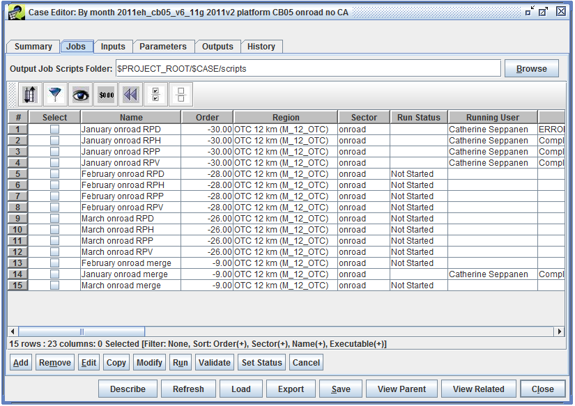
At the top of the Jobs tab is the Output Job Scripts Folder. When a job is run, the EMF creates a shell script in this folder. See Section 2.2 for more information about the script that the EMF writes and executes. Click the Browse button to set the scripts folder location on the EMF server. Otherwise, the folder location can be typed in the text field.
As shown in Figure 2-8, the Output Job Scripts Folder can use variables to refer to case settings or parameters. In this case, the folder location is set to $PROJECT_ROOT/$CASE/scripts. PROJECT_ROOT is a case parameter defined in the Parameters tab with the value /data/em_v6.2/2011platform. The CASE variable refers to the case’s abbreviation: test_2011eh_cb05_v6_11g. Thus, the scripts for the jobs in the case will be written to the folder /data/em_v6.2/2011platform/test_2011eh_cb05_v6_11g/scripts.
To view the details of a particular job, select the job, then click the Edit button to bring up the Edit Case Job window (Figure 2-9).
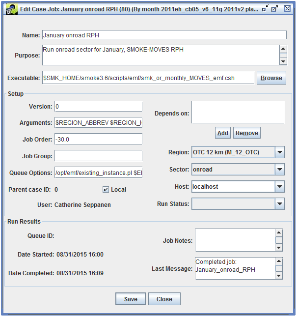
Table 2-6 describes each field in the Edit Case Job window.
| Name | Description |
|---|---|
| Name | The name of the job. When setting up a job, the combination of the job’s name, region, and sector must be unique. |
| Purpose | A short description of the job’s purpose or functionality. |
| Executable | The script or program the job will run. |
| Setup | |
| Version | Can be used to mark the version of a particular job. |
| Arguments | A string of arguments to pass to the executable when the job is run. |
| Job Order | The position of this job in the list of jobs. |
| Job Group | Can be used to label related jobs. |
| Queue Options | Any commands that are needed when submitting the job to run (i.e. queueing system options, or a wrapper script to call). |
| Parent case ID | If this job was copied from a different case, shows the parent case’s ID. |
| Local | Can be used to indicate to other users if the job runs locally vs. remotely. |
| Depends on | TBA |
| Region | Indicates the region associated with the job. |
| Sector | Indicates the sector associated with the job. |
| Host | If set to anything other than localhost, the job is executed via SSH on the remote host. |
| Run Status | Shows the run status of the job. |
| Run Results | |
| Queue ID | Shows the queueing system ID, if the job is run on a system that provides this information. |
| Date Started | The date and time the job was last started. |
| Date Completed | The date and time the job completed. |
| Job Notes | User editable notes about the job run. |
| Last Message | The most recent message received while running the job. |
After making any edits to the job, click the Save button to save the changes. The Close button closes the Edit Case Job window.
To create a new job, click the Add button to open the Add a Job window as shown in Figure 2-10.
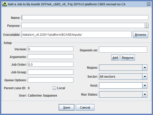
The Add a Job window has the same fields as the Edit Case Job window except that the Run Results section is not shown. See Table 2-6 for more information about each input field. Once the job information is complete, click the Save button to save the new job. Click Cancel to close the Add a Job window without saving the new job.
An existing job can be copied to a different case or the same case using the Copy button. Figure 2-11 shows the window that opens when copying a job.

If multiple jobs need to be edited with the same changes, the Modify button can be used. This action opens the window shown in Figure 2-12.
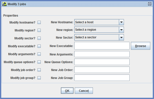
In the Modify Jobs window, check the checkbox next to each property to be modified. Enter the new value for the property. After clicking OK, the new value will be set for all selected jobs.
In the Jobs tab of the Case Editor window, the Validate button can be used to check the inputs for a selected job. The validation process will check each input for the job and report if any inputs use a non-final version of their dataset, or if any datasets have later versions available. If no later versions are found, the validation message “No new versions exist for selected inputs.” is displayed.
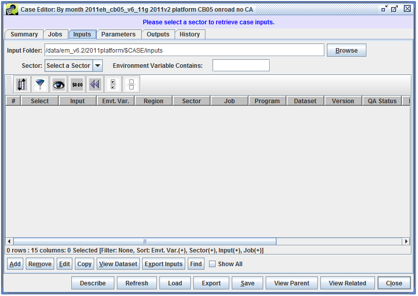
When the Inputs tab is initially viewed, the list of inputs will be empty as seen in Figure 2-13.
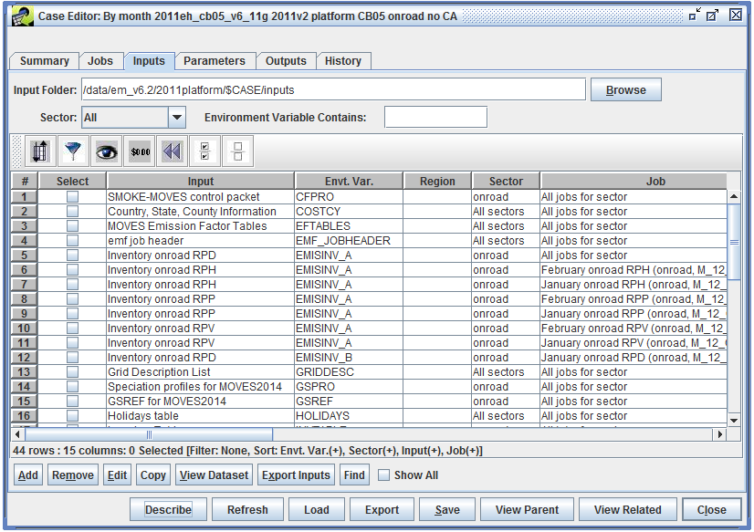
To view the inputs, use the Sector pull-down menu to select a sector associated with the case. In Figure 2-14, the selected sector is All, so that all inputs for the case are displayed.
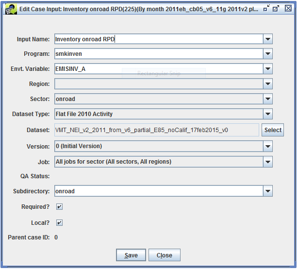
To view the details of an existing input, select the input, then click the Edit button to open the Edit Case Input window as shown in Figure 2-15.
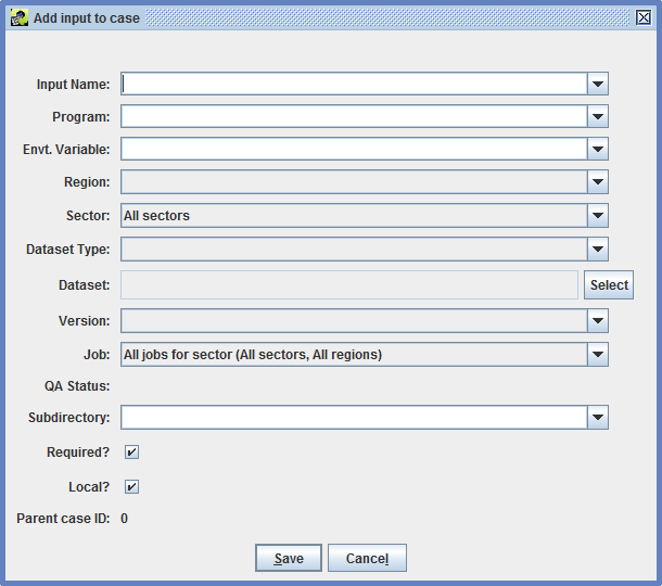
To create a new input, click the Add button to bring up the Add Input to Case window (Figure 2-16).
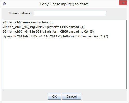
The Copy button can be used to copy an existing input to a different case. Figure 2-17 shows the Copy Case Input window that opens when the Copy button is clicked.
To view the dataset associated with a particular input, click the View Dataset button to open the Dataset Properties View window for the selected input.
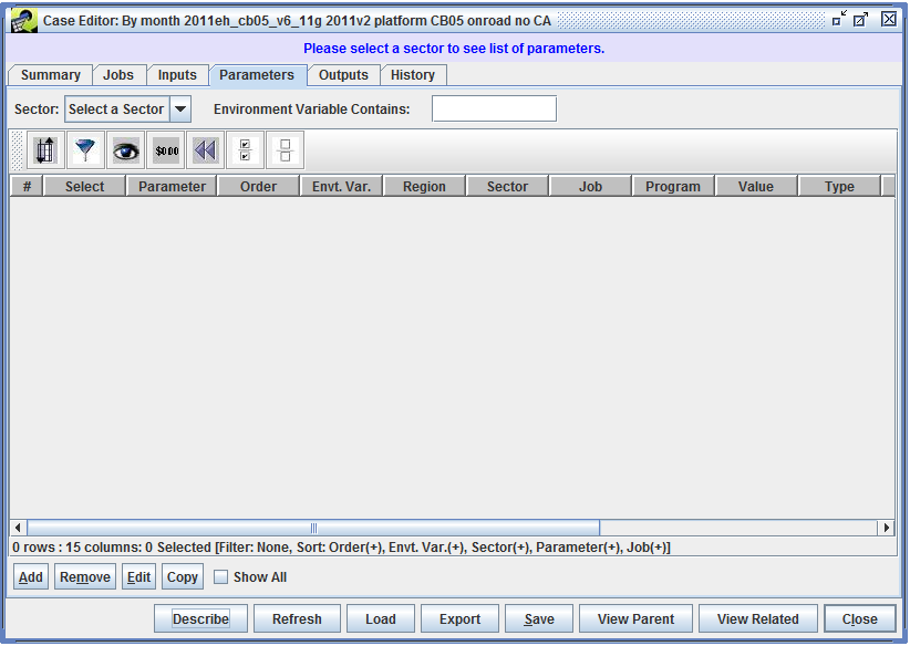
Like the Inputs tab, the Parameters tab will be empty when initially viewed, as shown in Figure 2-18.
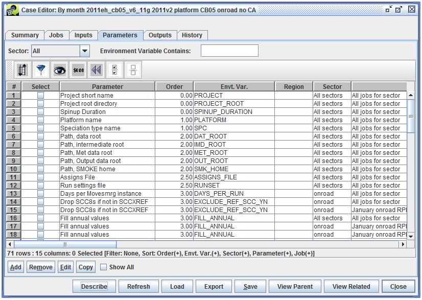
To view the parameters, use the Sector pull-down menu to select a sector. Figure 2-19 shows the Parameters tab with the sector set to All, so that all parameters for the case are shown.
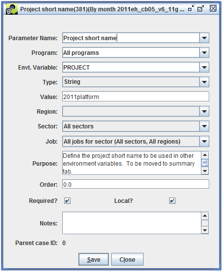
To view or edit the details of an existing parameter, select the parameter, then click the Edit button. This opens the parameter editing window as shown in Figure 2-20.
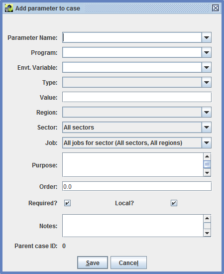
To create a new parameter, click the Add button and the Add Parameter to Case window will be displayed (Figure 2-21).
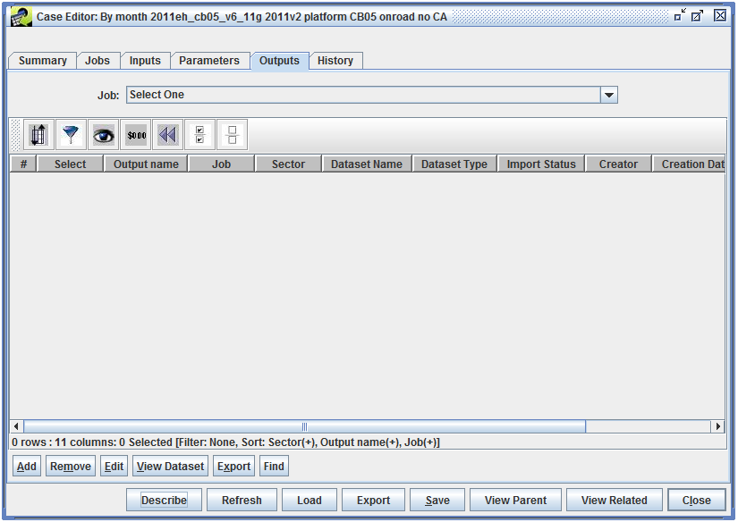
When initially viewed, the Outputs tab will be empty, as seen in Figure 2-22.
Use the Job pull-down menu to select a particular job and see the outputs for that job, or select “All (All sectors, All regions)” to view all the available outputs. Figure 2-23 shows the Outputs tab with All selected.
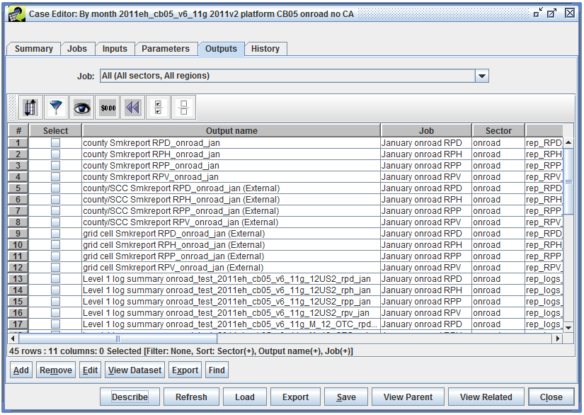
Table 2-7 lists the columns in the table of case outputs. Most outputs are automatically registered when a case job is run, and the job script is responsible for setting the output name, dataset information, message, etc.
| Column | Description |
|---|---|
| Output Name | The name of the case output. |
| Job | The case job that created the output. |
| Sector | The sector associated with the job that created the output. |
| Dataset Name | The name of the dataset for the output. |
| Dataset Type | The dataset type associated with the output dataset. |
| Import Status | The status of the output dataset import. |
| Creator | The user who created the output. |
| Creation Date | The date and time when the output was created. |
| Exec Name | If set, indicates the executable that created the output. |
| Message | If set, a message about the output. |
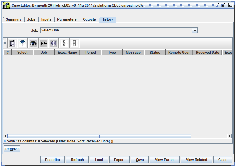
Like the Outputs tab, the History tab is empty when initially viewed (Figure 2-24).
The history of a single job can be viewed by selecting that job from the Job pull-down menu, or the history of all jobs can be viewed by selecting “All (All sectors, All regions)”, as seen in Figure 2-25.
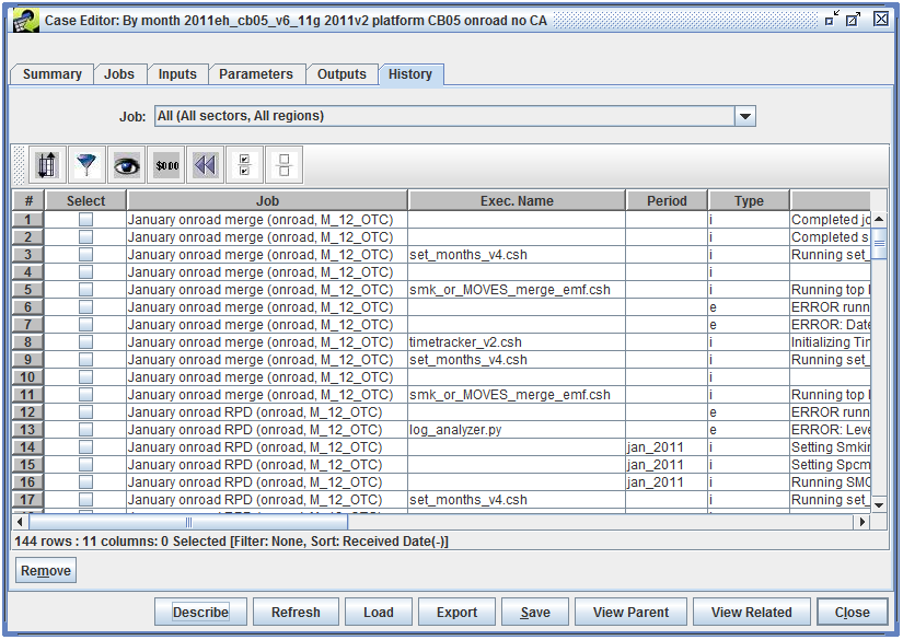
Messages in the History tab are automatically generated by the scripts that run for each case job. Each message will be associated with a particular job and the History tab will show when the message was received. Additionally, each message will have a type: i (info), e (error), or w (warning). The case job may report a specific executable and executable path associated with the message.
When a job is run, the EMF creates a shell script that will call the job’s executable. This script is created in the Output Job Scripts Folder specified in the Jobs tab of the Case Editor.
If the case includes an EMF_JOBHEADER input, the contents of this dataset are put at the beginning of the shell script. Next, all the environment variables associated with the job are exported in the script. Finally, the script calls the job’s executable with any arguments and queue options specified in the job.
In addition to the environment variables associated with a job’s inputs and parameters, Table 2-8 and Table 2-9 list the case and job settings that are automatically added to the script written by the EMF.
| Case Setting | Env. Var. | Example |
|---|---|---|
| abbreviation | $CASE | test_2011eh_cb05_v6_11g |
| base year | $BASE_YEAR | 2011 |
| future year | $FUTURE_YEAR | 2011 |
| model name and version | $MODEL_LABEL | SMOKE3.6 |
| downstream model | $EMF_AQM | CMAQ v5.0.1 |
| speciation | $EMF_SPC | cmaq_cb05_soa |
| start date & time | $EPI_STDATE_TIME | 2011–01–01 00:00:00.0 |
| end date & time | $EPI_ENDATE_TIME | 2011–12–31 23:59:00.0 |
| parent case | $PARENT_CASE | 2011eh_cb05_v6_11g_onroad_no_ca |
| Job Setting | Env. Var. | Example |
|---|---|---|
| sector | $SECTOR | onroad |
| job group | $JOB_GROUP | |
| region | $REGION | OTC 12 km |
| region abbreviation | $REGION_ABBREV | M_12_OTC |
| region gridname | $REGION_IOAPI_GRIDNAME | M_12_OTC |
The base MOVES2014 case is named “2011eh_cb05 emission factors”. Each job in the case generates emission factors for a single reference county, following these steps:
| Name | Purpose |
|---|---|
| 01073 - Jefferson County, AL | Run MOVES2014 for Jefferson County, AL |
| 01097 - Mobile County, AL | Run MOVES2014 for Mobile County, AL |
| 01101 - Montgomery County, AL | Run MOVES2014 for Montgomery County, AL |
| 01117 - Shelby County, AL | Run MOVES2014 for Shelby County, AL |
| Env. Var. | Description | Dataset Name |
|---|---|---|
| EMF_JOBHEADER | EMF job header for scripts | marama_amazon_emf_job_header |
| METFILE | RPD, RPV, and RPH meteorology data | MOVES_RH_DAILY_2011eg_v6_11g_12US2_2011001–2011365 |
| POLLUTANT_FORMULAS | Formulas for calculating additional emission factors | pollutant_formulas_AQ |
| POLLUTANT_MAPPING | Mapping from MOVES2014 pollutant IDs to SMOKE names | pollutant_mapping_AQ_CB05 |
| PROCESS_AGG | Emission process aggregation | process_aggregation |
| PROCESS_AGG_RPV | Emission process aggregation for RPV | process_aggregation_rpv |
| RPMETFILE | RPP meteorology data | MOVES_DAILY_2011eg_v6_11g_12US2_2011001–2011365 |
| Env. Var. | Description | Job | Dataset Name |
|---|---|---|---|
| COUNTY_DB | County-level inputs for MOVES2014 | 01073 - Jefferson County, AL | 01073 EPA default |
| 01097 - Mobile County, AL | 01097 EPA default | ||
| 01101 - Montgomery County, AL | 01101 EPA default | ||
| 01117 - Shelby County, AL | 01117 EPA default | ||
The EPA default county-level inputs started from the county database archive available at ftp://ftp.epa.gov/EmisInventory/2011v6/v2platform/2011emissions/onroad/2011RepCDBs–030115versions.zip. This archive contains sets of raw MySQL database files for each representative county. For example, the following files correspond to the database tables avgspeeddistribution and dayvmtfraction in the database named c01073y2011_20150301.
c01073y2011_20150301/avgspeeddistribution.frm
c01073y2011_20150301/avgspeeddistribution.MYD
c01073y2011_20150301/avgspeeddistribution.MYI
c01073y2011_20150301/dayvmtfraction.frm
c01073y2011_20150301/dayvmtfraction.MYD
c01073y2011_20150301/dayvmtfraction.MYI
After loading these databases into a local MySQL installation, the individual tables were dumped as CSV files using the exportMOVESCountyDB.sh script. This script produces the files listed in Table 3-1. The table also lists the MySQL table corresponding to each file and the corresponding tab in the MOVES County Data Manager window.
| File Name | MySQL Table Name | MOVES County Data Manager Tab |
|---|---|---|
| agedistribution.csv | sourcetypeagedistribution | Age Distribution |
| avgspeeddistribution.csv | avgspeeddistribution | Average Speed Distribution |
| dayvmtfraction.csv | dayvmtfraction | Vehicle Type VMT |
| fuelavft.csv | avft | Fuel |
| fuelformulation.csv | fuelformulation | Fuel |
| fuelsupply.csv | fuelsupply | Fuel |
| fuelusage.csv | fuelusagefraction | Fuel |
| hourvmtfraction.csv | hourvmtfraction | Vehicle Type VMT |
| hpmsvtypeyear.csv | hpmsvtypeyear | Vehicle Type VMT |
| imcoverage.csv | imcoverage | I/M Programs |
| monthvmtfraction.csv | monthvmtfraction | Vehicle Type VMT |
| population.csv | sourcetypeyear | Source Type Population |
| roadtypedistribution.csv | roadtypedistribution | Road Type Distribution |
The following case parameters can be used to control the MOVES2014 runs.
| Env. Var. | Description | Value |
|---|---|---|
| EMISSION_MODES | Determines which emissions modes are processed. Can be any combination of rate-per-distance (RPD), rate-per-vehicle (RPV), rate-per-profile (RPP), or rate-per-hour (RPH). | RPD, RPV, RPP, RPH |
| POLLUTANT_LIST | Determines which groups of pollutants to process. Can be any combination of OZONE, TOXICS, PM, or GHG. | OZONE, TOXICS, PM, GHG |
Section 4.5 describes how the SMOKE case integrates with Amazon Web Services. The MOVES2014 case is substantially the same. Each job has its Queue Options set as:
/opt/emf/launch_moves_instance.pl $EMF_JOBLOG
The launch_moves_instance.pl script performs the same tasks as the launch_instance.pl script described in Section 4.5. The only difference is that launch_moves_instance.pl finds a saved AMI whose description is “MOVES Node Template”.
The “MOVES Node Template” AMI has both MOVES2014 (October 2014) and MOVES2014a (December 2015) installed in /opt/MOVES2014 and /opt/MOVES2014a, respectively. See the SMOKE-MOVES wiki page Installing MOVES2014a on Linux.
MOVES2014 uses the default database named movesdb20141021cb6v2, while MOVES2014a uses movesdb20151028. Both databases are loaded in the template image. The SMOKE-MOVES scripts runspec_generator.pl and moves2smkEF.pl are located in /opt/SMOKE-MOVES/scripts. Instances created from this AMI automatically mount the /data directory from the EMF server.
In the Parameters tab, find the parameter “Path, MOVES2014 home” where the environment variable is MOVES_ROOT. To run MOVES2014, set the parameter’s value to /opt/MOVES2014. For MOVES2014a, change the parameter’s value to /opt/MOVES2014a. For clarity, the model and version set for the case in the Summary tab can be changed as well.
The base SMOKE processing case is named “By month 2011eh_cb05_v6_11g 2011v2 platform CB05 onroad no CA”. This case runs SMOKE for each emission factor type (RDP, RPV, RPP, and RPH) for each month of the year. After all four emission factor types have been processed for a single month, a job runs to merge the gridded outputs created by each individual job into a single set of outputs for the month.
| Name | Purpose |
|---|---|
| January onroad RPD | Run onroad sector for January, SMOKE-MOVES RPD |
| January onroad RPH | Run onroad sector for January, SMOKE-MOVES RPH |
| January onroad RPP | Run onroad sector for January, SMOKE-MOVES RPP |
| January onroad RPV | Run onroad sector for January, SMOKE-MOVES RPV |
| January onroad merge | Merge January RPD/RPP/RPV/RPH onroad components together |
| February onroad RPD | Run onroad sector for February, SMOKE-MOVES RPD |
| February onroad RPH | Run onroad sector for February, SMOKE-MOVES RPH |
| February onroad RPP | Run onroad sector for February, SMOKE-MOVES RPP |
| February onroad RPV | Run onroad sector for February, SMOKE-MOVES RPV |
| February onroad merge | Merge February RPD/RPP/RPV/RPH onroad components together |
| remaining months onroad RPD | Run onroad sector for month, SMOKE-MOVES RPD |
| remaining months onroad RPH | Run onroad sector for month, SMOKE-MOVES RPH |
| remaining months onroad RPP | Run onroad sector for month, SMOKE-MOVES RPP |
| remaining months onroad RPV | Run onroad sector for month, SMOKE-MOVES RPV |
| remaining months onroad merge | Merge month RPD/RPP/RPV/RPH onroad components together |
| SMOKE Env. Var. | Description | Dataset Name |
|---|---|---|
| CFPRO | Hourly emission factor adjustments | cfpro_zeroout_Colo_gas_rfl_except_11_counties_14nov2014_v0 |
| COSTCY | Country, state, and county information | costcy_for_2007platform_05jan2015_v11 |
| EFTABLES | MOVES2014 emission factor tables | EFTABLES_2011v2_MOVES2014_AQ_CB05_18feb2015 |
| EMF_JOBHEADER | EMF job header for scripts | marama_amazon_emf_job_header |
| GRIDDESC | Grid description | GRIDDESC_OTC |
| GSPRO | Speciation profiles | gspro_MOVES2014_CB5_draft_11dec2014_v6 |
| GSREF | Speciation cross-reference | testing_gsref_MOVES2014_dummy_nei_17nov2014_v2 |
| HOLIDAYS | Holidays list | holidays_04may2006_v0 |
| INVTABLE | Inventory data assignment table | invtable_MOVES2014_25sep2014_nf_v1 |
| MCXREF | Reference county cross-reference | MCXREF_2011eg_22aug2014_v0 |
| METMOVES | Temperature profiles | SMOKE_DAILY_2011eg_v6_11g_M_12_OTC_2011001–2011365 |
| MFMREF | Reference county fuel month cross-reference | MFMREF_2011eg_22aug2014_v0 |
| MGREF | Gridding surrogate cross-reference | mgref_us_2011v2platform_DRAFT_onroad_28jan2015_v2 |
| MRGDATE_FILES | Representative dates list | merge_dates_2011 |
| MTPRO_HOURLY | Hourly temporal profiles | mtpro_hourly_moves2014_23oct2014_13nov2014_v1 |
| MTPRO_MONTHLY | Monthly temporal profiles | amptpro_for_2011_platform_with_carb_mobile_2011CEM_moves_13aug2013_v0_tpro_monthly_13aug2014_v0 |
| MTPRO_WEEKLY | Weekly temporal profiles | mtpro_weekly_moves2014_17oct2014_13nov2014_v2 |
| MTREF | Temporal cross-reference | mtref_onroad_moves2014_23oct2014_28jan2015_v3 |
| REPCONFIG_GRID | Report configuration, gridded | repconfig_onroad_invgrid_2011platform_18aug2014_v1 |
| REPCONFIG_INV | Report configuration, inventory | repconfig_onroad_inv_2011platform_11may2011_v0 |
| SCCDESC | SCC descriptions | sccdesc_pf31_05jan2015_v22 |
| SPDPRO | Hourly speed profiles | SPDPRO_NEI_v2_2011_18sep2014_v0 |
| SRGDESC | Gridding surrogate descriptions | srgdesc_CONUS12_2010_v5_12nov2014_v4 |
| SRGPRO | Gridding surrogates | CONUS12_2010_v5_20141015 |
| SMOKE Env. Var. | Description | Job | Dataset Name |
|---|---|---|---|
| EMISINV_A | Activity inventory | All | VMT_NEI_v2_2011_from_v6_partial_E85_noCalif_17feb2015_v0 |
| January onroad RPP | VPOP_NEI_v2_2011_from_v5_partial_E85_noCalif_17feb2015_v0 | ||
| February onroad RPP | VPOP_NEI_v2_2011_from_v5_partial_E85_noCalif_17feb2015_v0 | ||
| remaining months onroad RPP | VPOP_NEI_v2_2011_from_v5_partial_E85_noCalif_17feb2015_v0 | ||
| January onroad RPV | VPOP_NEI_v2_2011_from_v5_partial_E85_noCalif_17feb2015_v0 | ||
| February onroad RPV | VPOP_NEI_v2_2011_from_v5_partial_E85_noCalif_17feb2015_v0 | ||
| remaining months onroad RPV | VPOP_NEI_v2_2011_from_v5_partial_E85_noCalif_17feb2015_v0 | ||
| January onroad RPH | HOTELING_NEI_v2_2011_from_v2_noCalif_16dec2014_v1 | ||
| February onroad RPH | HOTELING_NEI_v2_2011_from_v2_noCalif_16dec2014_v1 | ||
| remaining months onroad RPH | HOTELING_NEI_v2_2011_from_v2_noCalif_16dec2014_v1 | ||
| EMISINV_B | Second activity inventory | January onroad RPD | SPEED_NEI_v2_2011_from_v7_partial_E85_noCalif_17feb2015_v0 |
| Februrary onroad RPD | SPEED_NEI_v2_2011_from_v7_partial_E85_noCalif_17feb2015_v0 | ||
| remaining months onroad RPD | SPEED_NEI_v2_2011_from_v7_partial_E85_noCalif_17feb2015_v0 | ||
| MEPROC | Emission processes and pollutants | All | meproc_MOVES2014_RPD_AQ_17nov2014_v5 |
| January onroad RPP | meproc_MOVES2014_RPP_AQ_17nov2014_v2 | ||
| February onroad RPP | meproc_MOVES2014_RPP_AQ_17nov2014_v2 | ||
| remaining months onroad RPP | meproc_MOVES2014_RPP_AQ_17nov2014_v2 | ||
| January onroad RPV | meproc_MOVES2014_RPV_AQ_17nov2014_v5 | ||
| February onroad RPV | meproc_MOVES2014_RPV_AQ_17nov2014_v5 | ||
| remaining months onroad RPV | meproc_MOVES2014_RPV_AQ_17nov2014_v5 | ||
| January onroad RPH | meproc_MOVES2014_RPH_AQ_17nov2014_v6 | ||
| February onroad RPH | meproc_MOVES2014_RPH_AQ_17nov2014_v6 | ||
| remaining months onroad RPH | meproc_MOVES2014_RPH_AQ_17nov2014_v6 | ||
| MRCLIST | Emission factor table list | All | mrclist_RPD_2011v2_AQ_CB05_18feb2015_18feb2015_v0 |
| January onroad RPP | mrclist_RPP_2011v2_AQ_CB05_18feb2015_18feb2015_v0 | ||
| February onroad RPP | mrclist_RPP_2011v2_AQ_CB05_18feb2015_18feb2015_v0 | ||
| remaining months onroad RPP | mrclist_RPP_2011v2_AQ_CB05_18feb2015_18feb2015_v0 | ||
| January onroad RPV | mrclist_RPV_2011v2_AQ_CB05_18feb2015_18feb2015_v0 | ||
| February onroad RPV | mrclist_RPV_2011v2_AQ_CB05_18feb2015_18feb2015_v0 | ||
| remaining months onroad RPV | mrclist_RPV_2011v2_AQ_CB05_18feb2015_18feb2015_v0 | ||
| January onroad RPH | mrclist_RPH_2011v2_AQ_CB05_18feb2015_18feb2015_v0 | ||
| February onroad RPH | mrclist_RPH_2011v2_AQ_CB05_18feb2015_18feb2015_v0 | ||
| remaining months onroad RPH | mrclist_RPH_2011v2_AQ_CB05_18feb2015_18feb2015_v0 | ||
| SCCXREF | SCC8-to-SCC10 mapping | All | MOVES2014_SCCXREF_RPD_28jan2015_v5 |
| January onroad RPP | MOVES2014_SCCXREF_RPP_28jan2015_v3 | ||
| February onroad RPP | MOVES2014_SCCXREF_RPP_28jan2015_v3 | ||
| remaining months onroad RPP | MOVES2014_SCCXREF_RPP_28jan2015_v3 | ||
| January onroad RPV | MOVES2014_SCCXREF_RPV_28jan2015_v4 | ||
| February onroad RPV | MOVES2014_SCCXREF_RPV_28jan2015_v4 | ||
| remaining months onroad RPV | MOVES2014_SCCXREF_RPV_28jan2015_v4 | ||
| January onroad RPH | MOVES2014_SCCXREF_RPH_21jul2014_v0 | ||
| February onroad RPH | MOVES2014_SCCXREF_RPH_21jul2014_v0 | ||
| remaining months onroad RPH | MOVES2014_SCCXREF_RPH_21jul2014_v0 | ||
| Env. Var. | Description | Job | Value |
|---|---|---|---|
| MOVES_TYPE | Emissions mode to process in the job | month onroad RPD | RPD |
| month onroad RPH | RPH | ||
| month onroad RPP | RPP | ||
| month onroad RPV | RPV | ||
| USE_CONTROL_FACTORS | Apply factors to emissions in Movesmrg (defaults to N) | month onroad RPV | Y |
| EXCLUDE_REF_SCC_YN | Drop SCCs not in SCCXREF | All | N |
| month onroad RPP | Y | ||
| FILL_ANNUAL | Fill annual values when reading activity inventories | All | N |
| month onroad RPD | Y | ||
| month onroad RPH | Y | ||
Outputs from the various jobs and individual programs run by the jobs can be found in the following locations on the EMF server. All locations are relative to the case root directory /data/em_v6.2/2011platform/test_2011eh_cb05_v6_11g/.
| Description | Location | Example Filenames |
|---|---|---|
| Command-line output created when executing a job | scripts/logs |
January_onroad_RPD_M_12_OTC_test_2011eh_cb05_v6_11g_20150831183734_remote.log |
| Individual program logs | intermed/onroad/RPD/logsintermed/onroad/RPH/logsintermed/onroad/RPP/logsintermed/onroad/RPV/logs |
smkinven_RPD_onroad_jan_test_2011eh_cb05_v6_11g.log movesmrg_RPD_onroad_jan_test_2011eh_cb05_v6_11g_20110101_M_12_OTC_cmaq_cb05_soa.log |
| Per-mode model-ready output | intermed/onroad/RPDintermed/onroad/RPHintermed/onroad/RPPintermed/onroad/RPV |
emis_mole_RPD_onroad_20110101_M_12_OTC_cmaq_cb05_soa_test_2011eh_cb05_v6_11g_multiday.ncf |
| Inventory reports | reports/inv |
rep_RPD_onroad_jan_test_2011eh_cb05_v6_11g_inv_county_scc.txt |
| Temporalized inventory reports | reports/temporal |
rep_RPD_onroad_jan_test_2011eh_cb05_v6_11g_20110101_temporal_state_scc_srgid_M_12_OTC.txt |
| Movesmrg reports | reports/smkmerge/onroad/RPDreports/smkmerge/onroad/RPHreports/smkmerge/onroad/RPPreports/smkmerge/onroad/RPV |
rep_mole_RPD_onroad_20110101_M_12_OTC_cmaq_cb05_soa_test_2011eh_cb05_v6_11g.txt |
| Mrggrid program logs | intermed/onroad/logs |
mrggrid_onroad_test_2011eh_cb05_v6_11g_20110101_M_12_OTC_cmaq_cb05_soa.log |
| merged model-ready output | intermed/onroad |
emis_mole_onroad_20110101_M_12_OTC_cmaq_cb05_soa_test_2011eh_cb05_v6_11g.ncf |
Each job in the SMOKE case will run on its own Amazon EC2 instance. This is achieved using the Queue Options string, set for each job as:
/opt/emf/launch_instance.pl $EMF_JOBLOG
When a job is run, the EMF creates a shell script that exports all the case inputs and parameters, as described in Section 2.2. This shell script is passed as the final argument to the script specified by the Queue Options.
The launch_instance.pl script, specified in the job’s Queue Options, is a Perl script that creates and launches a new EC2 instance, then SSH’s into that instance and runs the EMF-created shell script. The EMF server itself runs on an EC2 instance with a custom Identity and Access Management (IAM) role named “launchComputeInstances”. This role is assigned the managed policy “AmazonEC2FullAccess” which allows launch_instance.pl to interact with EC2 instances.
launch_instance.pl performs the following steps:
The “Compute Node Template” AMI has the SMOKE executables and run scripts installed in /opt/smoke. EMF integration scripts are installed in /opt/emf. Instances created from this AMI automatically mount the /data directory from the EMF server.
An overview of the process can be found in the AWS documentation: Creating an Amazon EBS-Backed Linux AMI.
Start by launching an EC2 instance from the existing template. When choosing an AMI, select My AMIs and search for “Compute Node Template” to find the latest template. To match the instances that are automatically created when running a job, use the following settings:
| Setting | Value |
|---|---|
| Instance Type | m3.xlarge |
| Subnet | subnet-ea846b81 |
| Security Group | sg-c416f9ab |
All other settings use the default values. Note that the security settings will only allow SSH access to the compute node from the EMF server. The last step in launching the instance is to select an existing key pair or create a new key pair. If creating a new key pair, make sure to copy the private key to the EMF server and restrict the permissions. For example, if the private key file is named private_key.pem and stored in the ~/keys/ directory, the following command will disable access for all other users.
chmod go-rwx ~/keys/private_key.pem
Once the instance is running, make a note of the private IP address used by the instance. To find the private IP, switch to the Instances page in the AWS console and select the instance. Look for the Private IPs label in the bottom section. To access the instance, first SSH into the EMF server, then SSH to the new instance, specifying the private key, the private IP address, and the user ec2-user:
ssh -i ~/keys/private_key.pem ec2-user@private_ip
Once connected, update the instance as needed (run system updates, install new versions of software, etc.).
From the Instances page in the AWS web console, stop the running instance by selecting the instance, clicking the Actions button, and selecting Instance State, then Stop. Select the now stopped instance, click Actions, select Image, and then Create Image. In the pop-up window, name the image and set the image description as shown in Figure 4-1. Note that the image description is editable after the image has been created, while the image name is not.
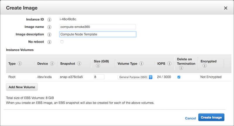
Click Create Image to start creating the new AMI.
Once the new AMI is created, make sure to either change the description on the old template image or delete the old image if it’s not needed. The next section describes how to delete an image. To update the description, start from the AMIs page in the AWS console. Use the search to find the old image by searching for “Compute Node Template”. Select the old image, then click the Edit button in the lower section. Change the Description field and then click Save. It’s important that there’s only one AMI with the description “Compute Node Template” so that when jobs run, the correct image is used to create the compute node instances.
To save on storage costs, the old compute node template can be removed by deregistering the AMI and deleting the EBS snapshot. See the AWS documentation: Deregistering Your AMI for more information; the compute node is an Amazon EBS-Backed AMI. From the AMIs page, first select the old AMI and make a note of the AMI ID. Then click Actions, and Deregister. In the pop-up, click Continue.
Switch to the Snapshots page in the AWS console. Enter the AMI ID into the search field to find the snapshot that corresponds to the deleted AMI. Then select the snapshot, click Actions and Delete. In the pop-up, click Yes, Delete.
Once the new AMI has been created, the instance can be terminated. From the Instances page in the AWS web console, select the stopped instance. Then click the Actions button, select Instance State, and choose Terminate. In the pop-up window, click Yes, Terminate. This will terminate the instance and delete the EBS volume that was created when the instance was started.
In the Jobs tab of the case, find the 5 jobs that correspond to the month of interest. For example, to run January, find the jobs named:
The four emission mode jobs (RPD, RPH, RPP, and RPV) must be run before the merge job. To start a job, select it, then click the Run button. The system will check for any problems with the inputs and display a message indicating if any newer versions of input datasets exist. In the Confirm Running Jobs dialog, click Yes to start running the job.
When a job finishes, the Run Status will switch to Completed. If the job fails, check the job’s history in the History tab for errors.
Once the four emission mode jobs have finished, run the merge job (i.e. January onroad merge), to merge the four individual output files into one combined output.
On the Summary tab for the case, add the region to the case by clicking the Add button below the Regions box. If the region has already been set up in the EMF, select it from the list that appears. Otherwise, click the New button to create the region.
In the Jobs tab, select all the jobs in the case, then click the Modify button to edit all the jobs at once. Click the checkbox next to Modify region? and select the newly added region in the New region pull-down menu. Click OK to save the changes.
Update the input datasets GRIDDESC, METMOVES, and SRGPRO to point to datasets that correspond to the new grid.
If needed, update the MET_ROOT parameter to point to the meteorology data on the new grid. For RPD mode, SMOKE will read temperature data from files located in $MET_ROOT/$REGION_ABBREV/mcip_out/METCRO2D*.
The case named “2011 Met4moves M_12_OTC” runs Met4moves, a program that processes gridded, hourly meteorology data, and outputs files used by MOVES2014 and SMOKE. Met4moves reads a list of meteorology files that contain data for the time period of interest; extracts temperature and relative humidity data; and calculates minimum and maximum temperatures, temperature profiles, and average relative humidities for each reference county during the episode. The outputs from Met4moves are used when setting up MOVES2014 runs so that the calculated emission factors will cover the range of temperatures recorded during the episode.
The Met4moves case has one job named “Met4moves”, which runs the Met4moves program for the episode specified by the case. This job uses the run script run_met4moves.csh. The inputs, parameters, and outputs for the case are described below.
| Env. Var. | Description | Dataset Name |
|---|---|---|
| COSTCY | Country, state, and county information | costcy_for_2007platform_05jan2015_v11 |
| EMF_JOBHEADER | EMF job header for scripts | marama_amazon_emf_job_header |
| GRIDDESC | Grid description | GRIDDESC_OTC |
| MCXREF | Reference county cross-reference | MCXREF_2011eg_22aug2014_v0 |
| MFMREF | Reference county fuel month cross-reference | MFMREF_2011eg_22aug2014_v0 |
| SRGDESC | Gridding surrogate descriptions | srgdesc_CONUS12_2010_v5_12nov2014_v4 |
| SRGPRO | Gridding surrogates | CONUS12_2010_v5_20141015 |
Met4moves also requires a METLIST input, which is a file that lists the meteorology files to read. This list file is created by the run_met4moves.csh script by listing all the files whose name starts with METCOMBO in the directory specified by the MET_ROOT case parameter. To match the SMOKE case, the individual meteorology files are assumed to be in a subdirectory specifying the grid:
$MET_ROOT/$REGION_ABBREV/mcip_out/METCOMBO*
The meteorology files input to Met4moves must contain temperature, pressure, and water vapor mixing ratio data. The temperature variable name can be specified as a case parameter (TVARNAME), while pressure and mixing ratio are the variables PRES and QV, respectively. Typically, the temperature data comes from 2-D gridded meteorology data (i.e. METCRO2D), while the pressure and mixing ratio are from the 1st layer of 3-D gridded meteorology data (METCRO3D). This data must be combined into a single file to be processed by Met4moves. These METCOMBO files can be created from separate METCRO2D and METCRO3D files using the SMOKE utility program Metcombine. Running Metcombine is not part of the Met4moves case.
The following case parameters control the behavior of Met4moves.
| Env. Var. | Description | Value |
|---|---|---|
| MET_ROOT | Path to the METCOMBO meteorology files | /data/external/met/test |
| SRG_LIST | Spatial surrogate codes used for selecting grid cells for a county | 100,240 |
| TVARNAME | Temperature variable name from meteorology files | TEMP2 |
Other Met4moves settings are automatically configured based on the case.
| Env. Var. | Case Setting | Value |
|---|---|---|
| STDATE | Case start date (Start Date & Time from Summary tab) | 2011001 |
| ENDATE | Case end date (End Date & Time from Summary tab) | 2011001 |
| IOAPI_GRIDNAME_1 | Abbreviation for the region associated with the job | M_12_OTC |
| SRGPRO_PATH | Based on the location of the SRGPRO dataset | /data/external/surrogates/CONUS12_2010_v5_20141015/ |
When the Met4moves job is run, the three output files created by Met4moves are automatically registered as datasets in the EMF. These datasets can then be used as inputs to MOVES2014 or SMOKE cases.
| Env. Var. | Dataset Type | Dataset Name |
|---|---|---|
| SMOKE_OUTFILE | Meteorology Temperature Profiles (External) | SMOKE_M_12_OTC_2011001_2011001.ncf |
| MOVES_OUTFILE | MOVES2014 Meteorology RPP | MOVES_M_12_OTC_2011001_2011001.txt |
| MOVES_RH_OUTFILE | MOVES2014 Meteorology RPD, RPV, RPH | MOVES_RH_M_12_OTC_2011001_2011001.txt |
The Met4moves case uses the same Amazon Web Services integration as the SMOKE case, described in Section 4.5. The “Compute Node Template” AMI includes the Met4moves program in the SMOKE installation, and the run_met4moves.csh script.
Update the case Start Date & Time and End Date & Time settings on the Summary tab in the Edit Case window. For Met4moves, only the date portion of these settings will be used. Note that these settings need to be entered in local time in the EMF client and will be automatically converted to GMT. See Section 2.1.1 for more information.
Make sure that the METCOMBO files located in the MET_ROOT subdirectory contain data for all the hours in the episode.
On the Summary tab for the case, add the region to the case by clicking the Add button below the Regions box. If the region has already been set up in the EMF, select it from the list that appears. Otherwise, click the New button to create the region.
Edit the Met4moves job and use the Region pull-down menu to select the new region.
Update the input datasets GRIDDESC and SRGPRO to point to datasets that correspond to the new grid.
If needed, update the MET_ROOT parameter to point to the meteorology data on the new grid. Remember that the exact location of the meteorology files is $MET_ROOT/$REGION_ABBREV/mcip_out/METCOMBO*.