In this tutorial, you’ll create and run a temporal allocation using the temporal allocation module in the EMF. Along the way, we’ll look at the various datasets that get used as inputs for a temporal allocation run and the datasets that get created as outputs of the run.
For our tutorial temporal allocation, we’ll estimate an average day emissions value for weekends in the first half of August 2011. We’ll look just at VOC emissions from a 2011 national point source EGU inventory.
The tutorial is split into three sections:
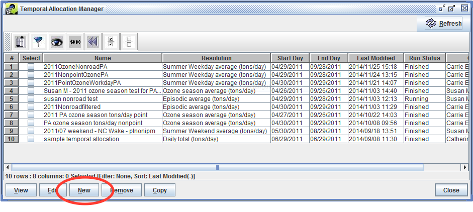
To get started, open the Manage menu from the main EMF window and select Temporal Allocation. You’ll see the Temporal Allocation Manager window which displays existing temporal allocation runs. Click the New button to start working on a new temporal allocation.
The Edit Temporal Allocation window will open, displaying the Summary tab.
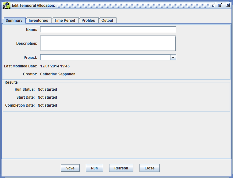
First, enter a Name for the temporal allocation like “August 2011 ptegu analysis - [your initials]”. Make sure to include your initials so that your temporal allocation has a unique name.
The Description is optional. You can use the description to describe what the temporal allocation will accomplish or the type of analysis you’re doing. For example:
Calculate average day VOC emissions for weekends in the first half of August 2011 for the ptegu sector
The Project is also optional. You might assign related temporal allocation runs to the same project to make finding and managing the runs easier. For now, you can leave the Project empty.
The Last Modified Date and Creator are automatically set by the EMF. The Results section is initially blank; it will display information once the temporal allocation has been run.
Click the Save button to save your new temporal allocation. If the name is not unique, you’ll see an error at the top of the window: “A Temporal Allocation named ‘August 2011 ptegu analysis’ already exists”. If needed, add some text to the name to make it unique and try saving again.
When your temporal allocation is saved, you’ll see the message “Temporal Allocation was saved successfully” at the top of the window. You can save your temporal allocation at any time as you’re editing it.
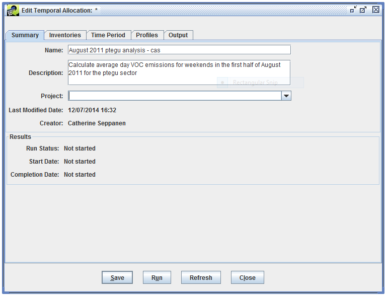
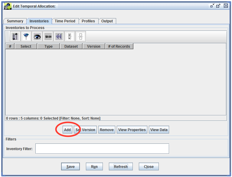
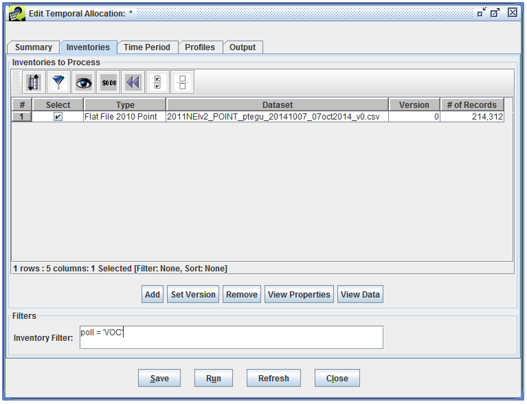
Next, we’ll select the inventory we want to process in our temporal allocation. Switch to the Inventories tab. This tab displays a list of the inventories for the temporal allocation. For our new temporal allocation, the list is currently empty. Click the Add button in the middle of the window.
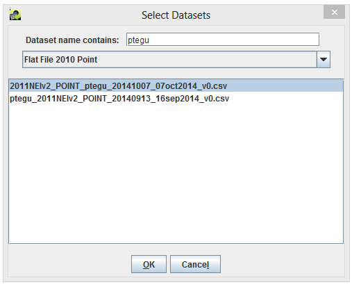
In the Select Datasets window that opens, use the Choose a dataset type pull-down menu to select the dataset type “Flat File 2010 Point”. You’ll then see a list of available Flat File 2010 Point datasets. In the Dataset name contains field, type in “ptegu” and hit the Enter key to narrow down the list. Click on the dataset named “2011NEIv2_POINT_ptegu_20141007_07oct2014_v0.csv” to select it, then click the OK button.
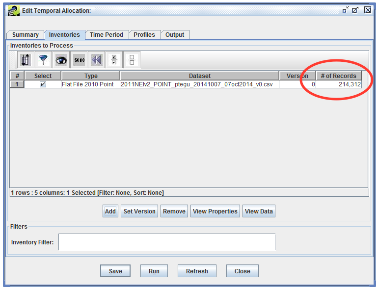
Back in the Inventories tab, you’ll now see your selected inventory listed. The list of inventories includes a column with the number of records in the dataset. This is useful to approximate how large your temporal allocation run will be if you don’t enter any filtering criteria. Our selected ptegu dataset has 214,312 records.
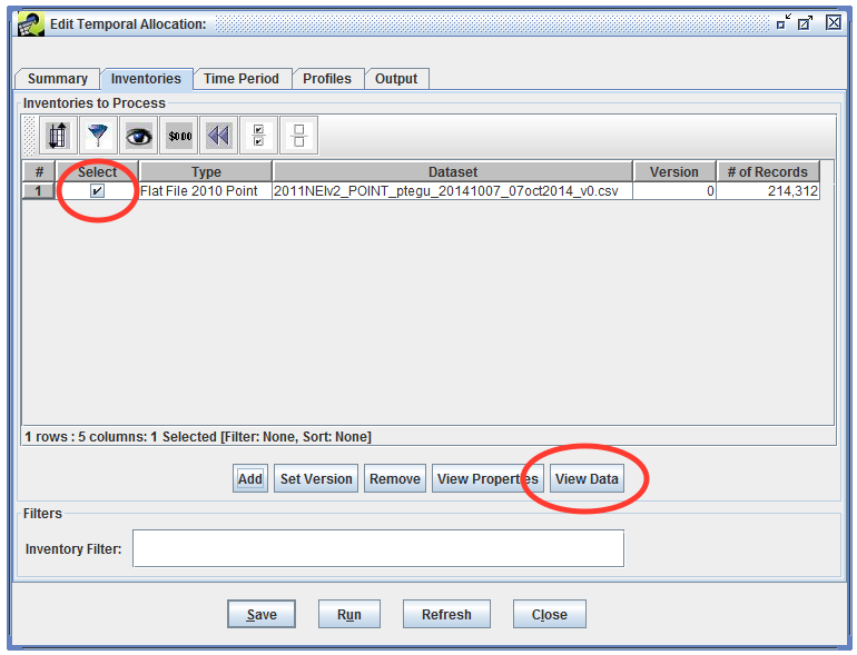
Let’s take a look at the inventory data and work out the filtering criteria we want to use. Check the checkbox next to the inventory dataset and then click the View Data button.
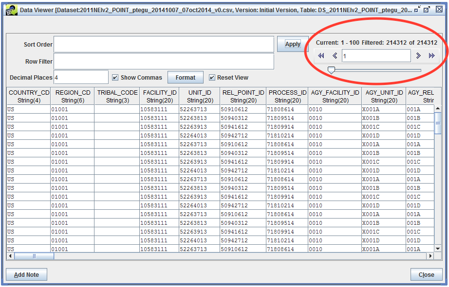
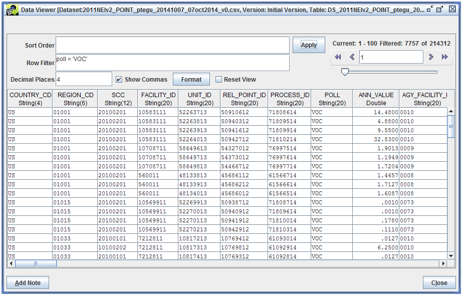
This opens the Data Viewer window with the raw data in the inventory dataset. We can use the Row Filter to try out different filtering options. The top right corner of the Data Viewer window shows a count of how many records match our filter. Currently, we don’t have a filter applied so our filtered count is 214,312, all the records in the dataset.
Remember that the Row Filter uses snippets of SQL from the WHERE clause. These snippets will generally look like
[column name] [operator] [value]
where [operator] might be =, >, LIKE, IN, etc. For instance, to match records where the region code is 01001, we can use the Row Filter
region_cd = '01001'
To match records where the SCC starts with 10, we could use a Row Filter
scc LIKE '10%'
For our temporal allocation, we’re only interested in VOC emissions, so enter the Row Filter
poll = 'VOC'
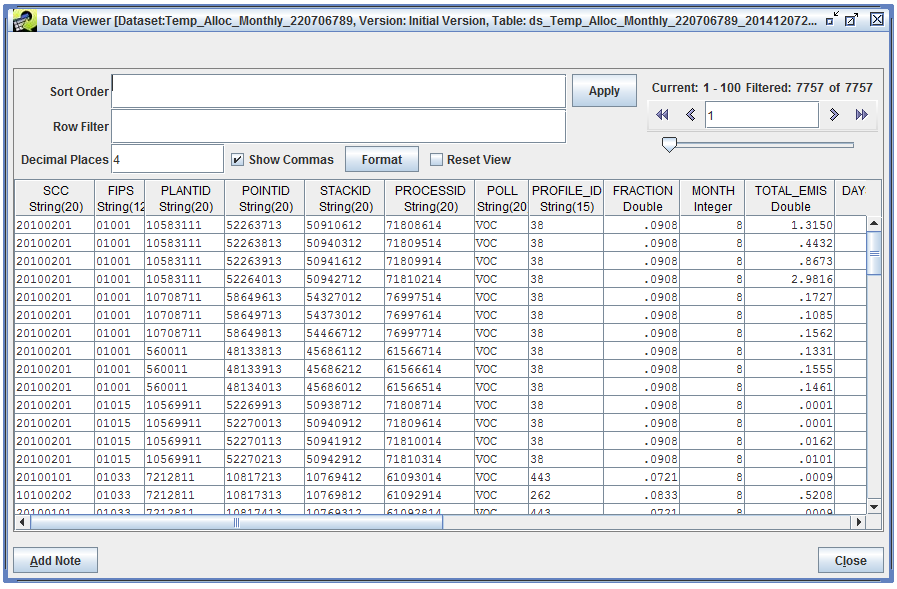
Click the Apply button to apply the filter. There are 7,757 records that match our filter criteria. Note that in the following screenshot, we’ve rearranged the columns to better show the source information (region, SCC, facility ID, etc.), pollutant, and emissions values.
Suppose we wanted to match records where the pollutant name starts with PM. In our inventory, that would be pollutants PM-CON, PM10-FIL, PM10-PRI, PM25-FIL, and PM25-PRI. What row filter could we use? [We could use either of the following filters:
poll LIKE 'PM%'poll IN ('PM-CON', 'PM10-FIL', 'PM10-PRI', 'PM25-FIL', 'PM25-PRI')]
To illustrate how the temporal allocation process works, we’ll pick a source from the inventory and track its emissions through the process. The following Row Filter matches just a single record:
region_cd = '01001' AND scc = '20100201' AND facility_id = '10583111' AND unit_id = '52263713' AND poll = 'VOC'
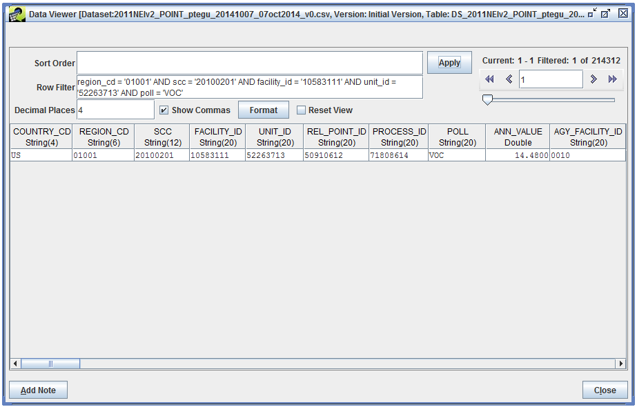
We’ll write down the source information and annual total VOC emissions for later.
| Region | 01001 |
| SCC | 20100201 |
| Facility ID | 10583111 |
| Unit ID | 52263713 |
| Annual VOC emissions | 14.48 tons/yr |
Close the Data Viewer window and return to the Inventories tab of the Edit Temporal Allocation window. Enter your filter criteria in the Inventory Filter field: poll = 'VOC'.
Switch to the Time Period tab. In this tab, we’ll set up the output resolution we want and the time period.
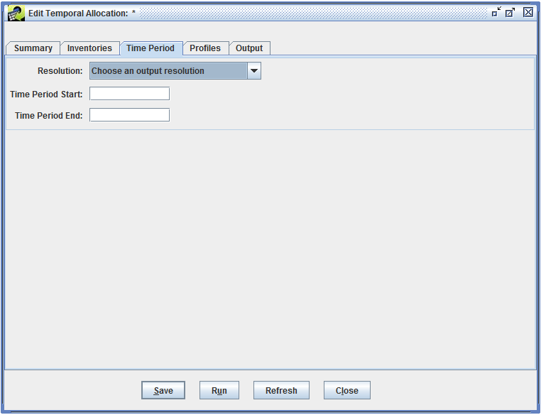
We want to estimate average day emissions for weekends, so in the Resolution pull-down menu, select “Episodic weekend average (tons/day)”. Our time period is the first half of August 2011; type in the Time Period Start as “08/01/2011” and the Time Period End as “08/15/2011”.
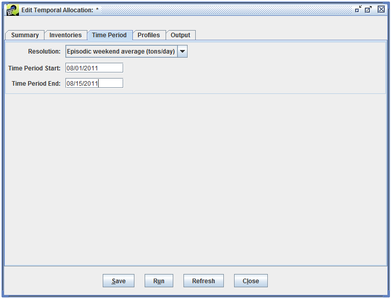
We when run the temporal allocation, the module will estimate emissions for each weekend day (Saturdays and Sundays) in our episode, then calculate an average day value across all the weekend days. Our episode has 4 weekend days (August 6th and 7th, and August 13th and 14th).
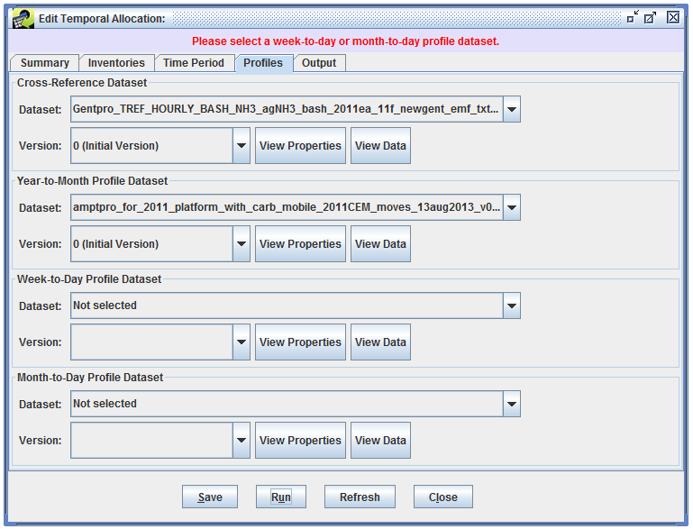
Now we’ll set up the cross-reference and profile datasets to use. Switch to the Profiles tab.
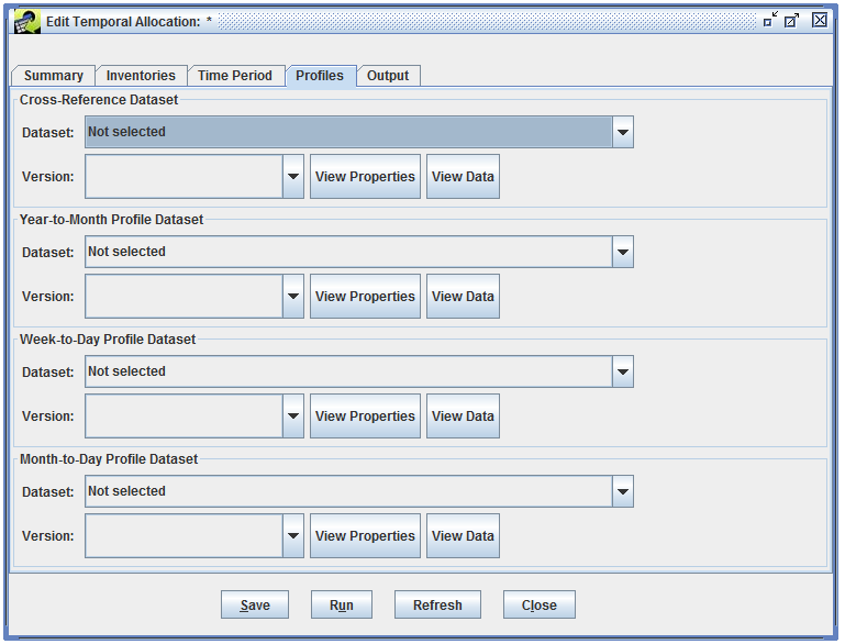
Because our inventory has annual data and we need to estimate daily totals, we’ll need to select a cross-reference dataset, a year-to-month profile dataset, and either a week-to-day or month-to-day profile dataset. Currently, the MARAMA system has datasets loaded from the EPA 2011 modeling platform. There is only one cross-reference dataset, one year-to-month profile dataset, and one week-to-day profile dataset loaded, so you’ll only see one option in each of the Dataset pull-down menus. There are no month-to-day profile datasets loaded.
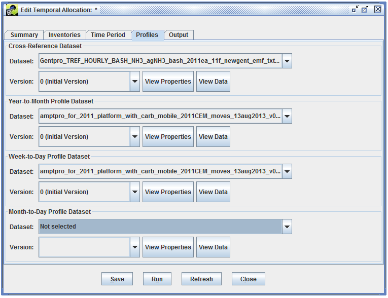
For the cross-reference dataset, year-to-month profile dataset, and week-to-day profile dataset, select the available dataset for each.
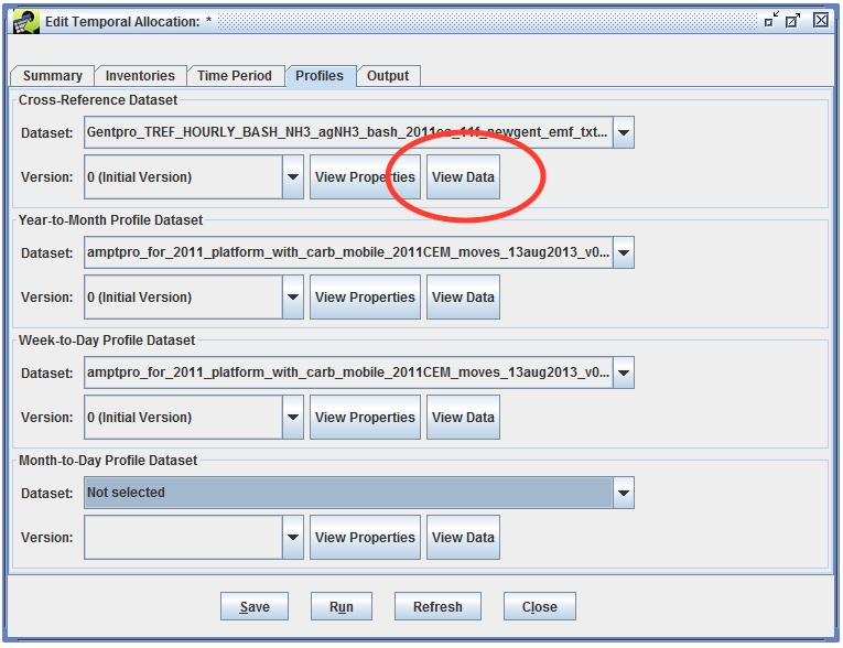
Let’s take a look at the underlying data in the datasets you selected. Click the View Data button for the Year-to-Month Profile Dataset.
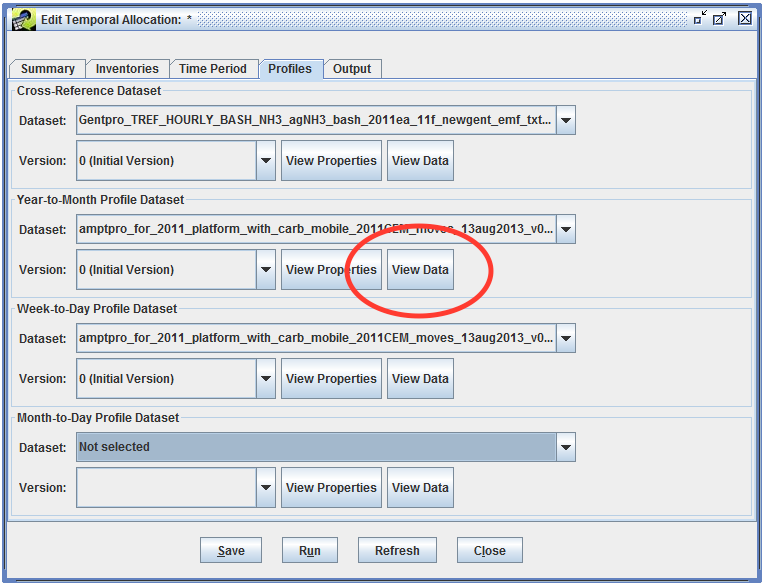
The Data Viewer opens, showing the data contained in the year-to-month profile dataset.
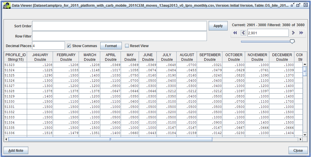
Each record in the year-to-month profile dataset consists of a profile ID and 12 factors, representing the fraction of annual emissions that should be allocated to each month of the year. The week-to-day profile dataset is very similar, only each record has 7 factors, one for each day of the week.
Now view the data in the Cross-Reference Dataset by clicking the corresponding View Data button.
A new Data Viewer window will open, showing the data in the cross-reference dataset.
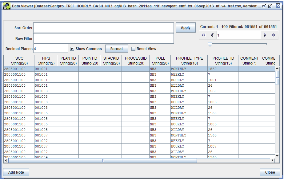
The cross-reference dataset is used to assign each source in the inventory a set of temporal profiles. A single cross-reference dataset is used to assign year-to-month, week-to-day, and month-to-day profiles.
The first 7 columns (SCC, FIPS, PLANTID, POINTID, STACKID, PROCESSID, and POLL) specify the source (or group of sources) in the inventory. The PROFILE_TYPE and PROFILE_ID columns indicate which profile the matched sources should use. Profile type MONTHLY indicates profiles in the year-to-month dataset, while profile type WEEKLY indicates profiles in the week-to-day dataset. Profile types HOURLY and ALLDAY indicate profiles to use when allocating emissions to individual hour in a day; the temporal allocation module doesn’t use this data.
For the highlighted row in the screenshot, this row will match any source with SCC = 280500110, FIPS code = 001001, and pollutant = NH3. Those matched sources will use the year-to-month profile with ID = 1560. The next line has the same source information and lists the week-to-day profile ID to use (ID 7).
After reviewing the cross-reference data, close the Data Viewer window and return to the Edit Temporal Allocation window. Be sure to save your temporal allocation by clicking the Save button at the bottom of the window.
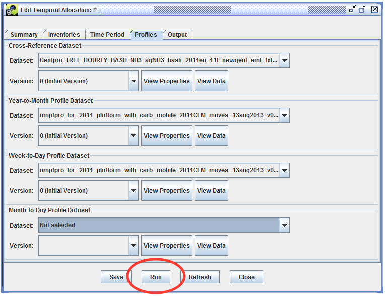
Now we’re ready to run the temporal allocation. Click the Run button at the bottom of the Edit Temporal Allocation window.
If there are any problems found with the values you’ve entered, you’ll need to fix them before your run starts. For instance, if you forgot to select the week-to-day profile dataset, you’ll see an error like so:
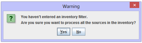
If you try to run a temporal allocation without entering an inventory filter, the EMF will ask you if you’re sure you want to process all the sources in the inventory. In our case, we entered an inventory filter (poll = 'VOC'), so we won’t see this prompt.
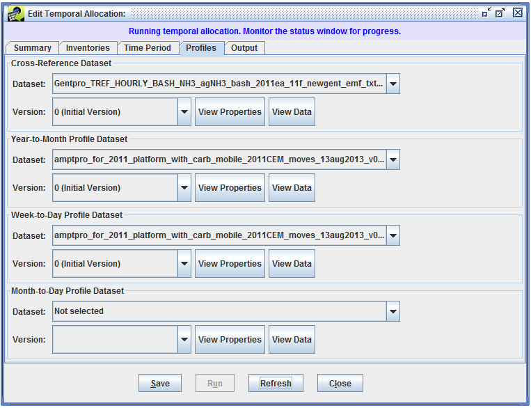
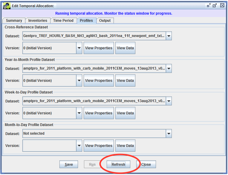
Once the run starts, you’ll see the message “Running temporal allocation. Monitor the status window for progress.” displayed at the top of the window.
While your temporal allocation is running, various messages will be displayed in the Status window.
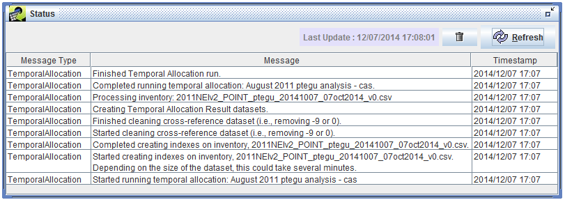
When your run has finished, you’ll see the message “Finished Temporal Allocation run.” in the Status window. For the tutorial example we’ve set up, the run should finish in about a minute.
In the Edit Temporal Allocation window, click the Refresh button to update the temporal allocation.
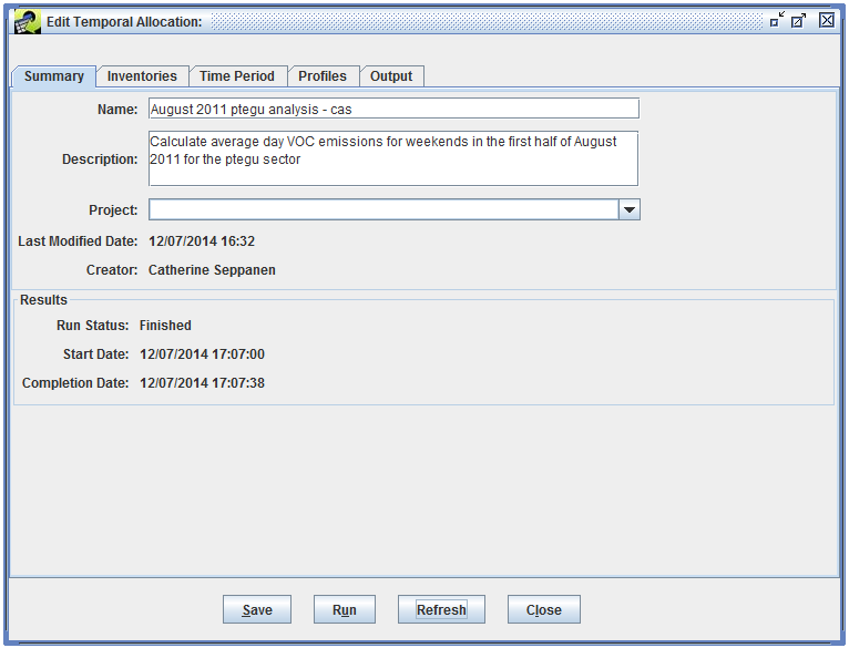
Switch to the Summary tab. The Results section will now show information about the most recent run.
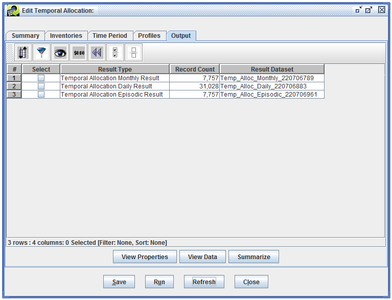
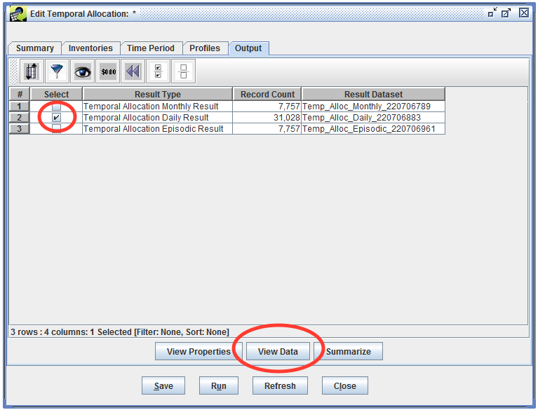
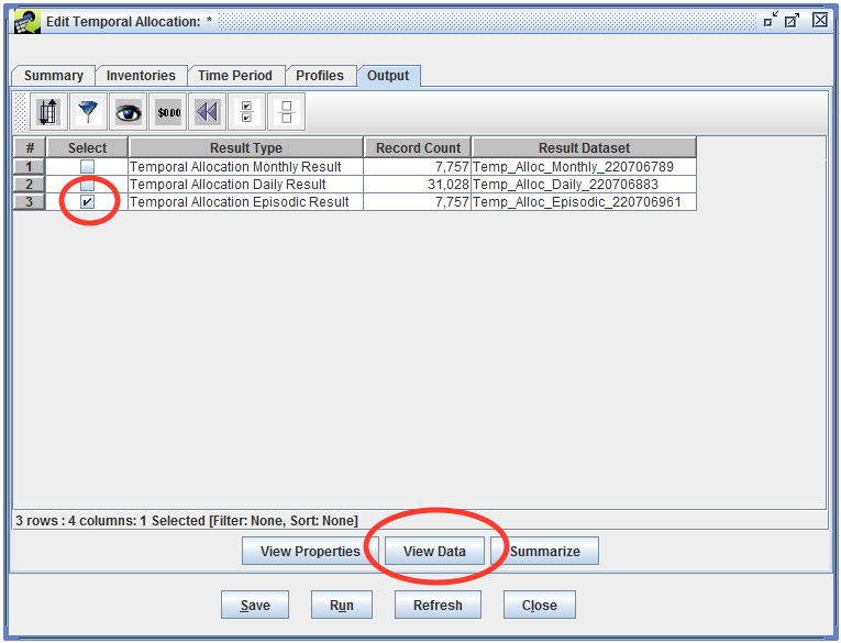
Now we’ll look at the outputs that were created when we ran the temporal allocation. Switch to the Output tab, where you’ll see three output datasets listed.
To understand the results datasets that have been created, let’s look at what the temporal allocation module needed to do during the run, starting from the annual emissions data in the inventory.
The three output datasets correspond to each of these steps.
| Result Type | Description |
|---|---|
| Temporal Allocation Monthly Result | Monthly total emissions for each source, for each month in the episode (i.e., August for our run) |
| Temporal Allocation Daily Result | Daily total emissions for each source, for each processed day in the episode (i.e., Saturdays and Sundays for our run) |
| Temporal Allocation Episodic Result | Episodic average day emissions for each source |
Remember the source that we picked out of the inventory?
| Region | 01001 |
| SCC | 20100201 |
| Facility ID | 10583111 |
| Unit ID | 52263713 |
| Annual VOC emissions | 14.48 tons/yr |
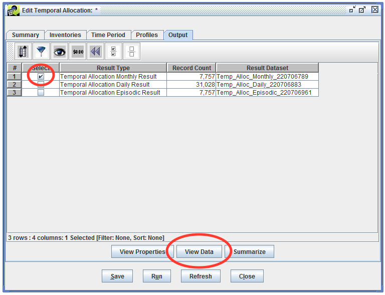
Let’s find the matching record in each of the output datasets. First, check the checkbox next to the Temporal Allocation Monthly Result, then click the View Data button.
The Data Viewer opens, displaying the data in the monthly result dataset.
We’ll use a Row Filter to find the source we’re interested in:
fips = '01001' AND scc = '20100201' AND plantid = '10583111' AND pointid = '52263713'
You may notice that the column names in our Row Filter are different from the inventory. See the Column Naming section in the Temporal Allocation Module User’s Guide for more info.
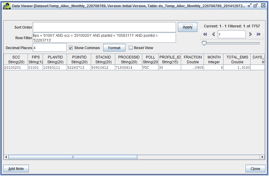
The PROFILE_ID column tells us which year-to-month profile was used for our source. The FRACTION column indicates the specific factor used for August. We multiply the source’s annual emissions by the monthly factor to calculate the total emissions in August (reported in the TOTAL_EMIS column).
14.48 tons/yr * 0.0908 yr/month = 1.315 tons/month
The monthly result dataset also includes monthly average day emissions (AVG_DAY_EMIS). These values are calculated by dividing the monthly total emissions by the number of days in the month (as reported in the DAYS_IN_MONTH column).
1.315 tons/month / 31 days/month = 0.0424 tons/day
Now that we’ve looked at the estimated monthly emissions, we’ll move on to the daily emissions for Saturdays and Sundays in our episode. Go back to the Edit Temporal Allocation window and view the data for the Temporal Allocation Daily Result.
The Data Viewer opens, displaying the data in the daily result dataset.
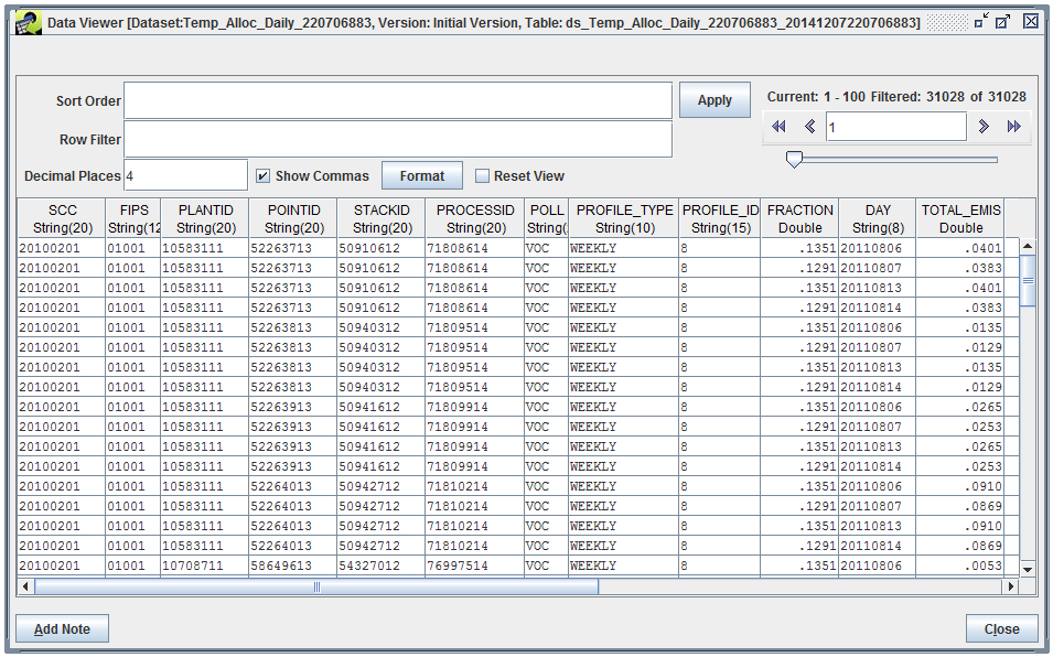
We’ll apply the same Row Filter to find our source:
fips = '01001' AND scc = '20100201' AND plantid = '10583111' AND pointid = '52263713'
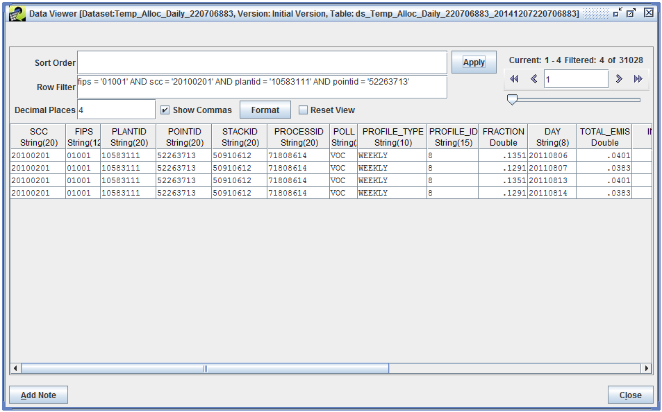
Since there are four days in our episode (two weekends), there are four records matched for our source. The DAY column contains the calendar date for each record. Just like the monthly results, the PROFILE_ID column tells us which profile was used for our source. Because daily estimates can use either week-to-day or month-to-day profiles, the PROFILE_TYPE column indicates which type of profile was used. Since we only used the week-to-day profile dataset, all the values in the column will be WEEKLY.
To apply a week-to-day profile, first we calculate a weekly total value starting from the monthly average day value:
0.0424 tons/day * 7 days/week = 0.2968 tons/week
Then, we can use the week-to-day fraction (reported in the FRACTION column) to estimate the day-specific emissions. For Saturday emissions:
0.2968 tons/week * 0.1351 days/week = 0.0401 tons/day
For Sunday emissions:
0.2968 tons/week * 0.1291 days/week = 0.0383 tons/day
The daily total emissions are reported in the TOTAL_EMIS column in the Temporal Allocation Daily Result dataset.
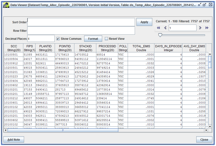
Finally, with the daily estimates calculated, the episodic average can be calculated. Let’s open the Temporal Allocation Episodic Result from the Output tab in the Edit Temporal Allocation window.
The Data Viewer opens, displaying the data in the episodic result dataset.
We’ll use the same Row Filter to find our source:
fips = '01001' AND scc = '20100201' AND plantid = '10583111' AND pointid = '52263713'
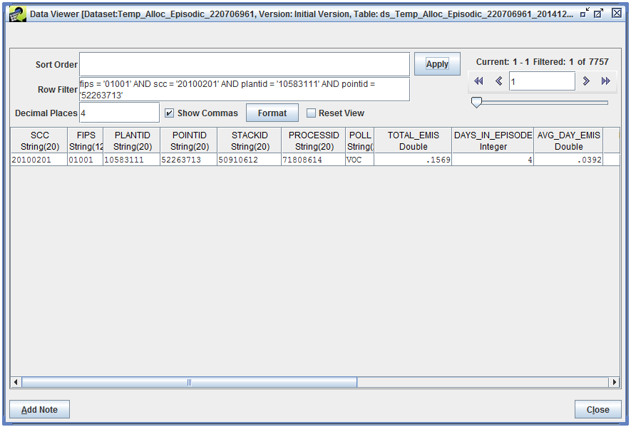
The TOTAL_EMIS column contains the summed emissions for all the days in the episode.
0.0401 tons/day [Aug. 6] + 0.0383 tons/day [Aug. 7] + 0.0401 tons/day [Aug. 13] + 0.0383 tons/day [Aug. 14] = 0.1569 tons/episode
The DAYS_IN_EPISODE column reports how many days are in the episode. While our episode start and end date covered 15 days (Aug. 1 through Aug. 15), we requested only weekend days be considered, so we have a total of 4 days in the episode. Finally, the column AVG_DAY_EMIS reports the episodic average day emissions for our source.
0.1569 tons/episode / 4 days/episode = 0.0392 tons/day
We stepped through the output for a single source in the inventory. The temporal allocation module repeats these calculations for every source in the inventory that matches our filter criteria.
You can also access the temporal allocation outputs from the Dataset Manager. From the main Manage menu, select Datasets to open the Dataset Manager window. Use the Show Datasets of Type pull-down menu to select the output result dataset type, e.g., “Temporal Allocation Episodic Result”.
The temporal allocation output datasets are automatically named with unique code. You can find the specific output dataset names listed in the Output tab of the Edit Temporal Allocation window. In the screenshots above, the name of the episodic result dataset is “Temp_Alloc_Episodic_220706961”. Note that rerunning a temporal allocation will cause the outputs to be regenerated with new names.
When you run a temporal allocation, you will be the creator of the output datasets. In the Dataset Manager window, you can look at the Creator column to find datasets you’ve created. You may need to scroll to the right to see the Creator column. You can also use the Advanced Dataset Search to find datasets that you’ve created.
In this tutorial, you created and ran a temporal allocation using the EMF. We started with annual emissions and calculated an average day value for weekends in our episode. We looked at the various datasets that go into a temporal allocation: the inventory itself, the cross-reference dataset, the year-to-month profile dataset, and the week-to-day profile dataset. We used an inventory filter to select a subset of records from the inventory to process. After running the temporal allocation, we looked at the three output datasets: monthly results, daily results, and episodic results. We saw how the temporal profiles are applied to calculate the estimated emissions at each step in the processing.