Last updated: June 11, 2019
This document is a user’s guide for the Control Strategy Tool (CoST) software. CoST was developed in cooperation between the University of North Carolina Institute for the Environment and the United States Environmental Protection Agency (EPA), Office of Air Quality Planning and Standards, Health and Environmental Impacts Division (HEID). CoST estimates the air pollution emissions reductions and costs associated with future-year control scenarios, and generates emissions inventories with the control scenarios applied Misenheimer, 2007; Eyth, 2008. CoST includes a database of information about emissions control measures, their costs, and the types of emissions sources to which they apply. The purpose of CoST is to support national- and regional-scale multi-pollutant analyses. CoST helps to develop control strategies that match control measures to emission sources using algorithms such as “Maximum Emissions Reduction” (for both single- and multiple-target pollutants) and “Least Cost”. CoST includes a graphical user interface (GUI) for configuring CoST simulations and viewing the results.
Results from a CoST control strategy run include the estimated cost and emissions (tons) reduction achieved for each control measure-source combination. CoST is an engineering cost estimation tool for creating controlled inventories and is not currently intended to model emissions trading strategies, nor is it an economic impact assessment tool. Control strategy results can be exported to comma-separated-values (CSV) files, Google Earth-compatible (.kmz) files, or Shapefiles. The CoST results can be viewed in the GUI as graphical tables that support sorting, filtering, and plotting. The Strategy Detailed Results from a CoST strategy run can be input to the Sparse Matrix Operator Kernel Emissions (SMOKE) modeling system, which is used by the EPA to prepare emissions inputs for air quality modeling.
CoST is a component of the Emissions Modeling Framework (EMF), which is currently being used by the EPA to solve many of the long-standing complexities of emissions modeling Houyoux, 2008. Emissions modeling is the process by which emissions inventories and other related information are converted to hourly, gridded, chemically speciated emissions estimates suitable for input into a regional air quality model such as the Community Multiscale Air Quality (CMAQ) model. The EMF supports the management and quality assurance of emissions inventories and emissions modeling-related data, and also the running of SMOKE to develop CMAQ inputs. Providing CoST as a tool integrated within the EMF facilitates a level of collaboration between control strategy development and emissions inventory modeling that was not previously possible. The concepts that have been added to the EMF for CoST are “control measures” and “control strategies.” Control measures store information about available control technologies and practices that reduce emissions, the source categories to which they apply, the expected control efficiencies, and their estimated costs. A control strategy is a set of control measures applied to emissions inventory sources (in addition to any controls that are already in place) to accomplish an emissions reduction goal. These concepts are discussed in more detail later in this document.
CoST is designed for multi-pollutant analyses and data transparency. It provides a wide array of options for developing emissions control strategies through the Control Measures Database (CMDB). The CoST GUI provides a graphical interface for accessing the CMDB, designing control strategies, and viewing the results from control strategy runs. CoST has been applied to develop strategies for criteria and hazardous air pollutants (HAPs). CoST has been used in some very limited analyses for greenhouse gases (GHGs). The main limiting factors in performing GHG analyses are the availability of (1) GHG emissions inventories with enough detail to support the application of control measures to individual sources or source groups, and (2) GHG control measures, with the associated technology implementation and costs.
The CoST algorithms for developing control strategies include:
This document provides information on how to use CoST to view and edit control measures and how to develop control strategies. This includes how to specify the input parameters to control strategies, how to run the strategies, and how to analyze the outputs from the strategies. The screenshots and examples in this guide were prepared using version 2.15 of CoST. For additional information on other aspects of CoST, please see the following independent documents:
These documents, and additional information about CoST, can be found at the EPA website on Cost Analysis Models/Tools for Air Pollution Regulations.
Because CoST is fully integrated within the EMF, installing CoST is the same as installing the EMF. There are two parts of the CoST/EMF system: a client and a server. In this guide, it is assumed that you need to install both the client and the server.
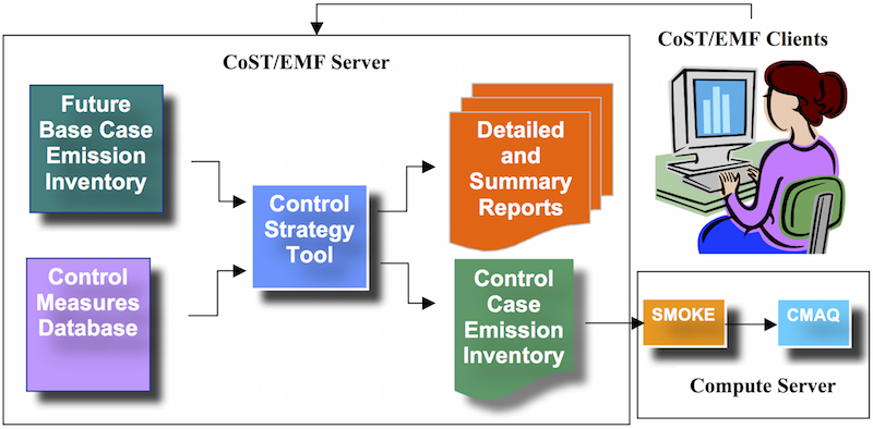
In the CoST client-server system, client software that runs on a desktop computer is used to connect to a server running the CoST algorithms and database. The CoST/EMF client is a Java program that accesses Java and PostgreSQL software running on the CoST/EMF server. CoST/EMF requires that a recent version of Java be installed on each user’s computer. The EMF database server stores information related to emissions modeling, including emissions inventory datasets and a database of emissions control measures. When a control strategy is developed, new datasets and summaries of them are created within CoST, and controlled emissions inventories can optionally be generated. These emissions inventories can be exported from CoST and then used as inputs to the SMOKE modeling system, which prepares emissions data for use in the CMAQ model. A schematic of the CoST/EMF client-server system see Figure 2.1.
The software installation package is a ZIP file (~300MB) that contains all the relevant supporting applications and software required to run the CoST system on a Windows-based machine. The installation package also contains the most recent version of the CMDB available at the time of the software release. Instructions for optionally updating the CMDB are provided at the end of this section.
The CoST server requires Java Runtime Environment 8 or higher (also known as JRE 1.8), Tomcat and PostgreSQL. All of these components are in the CoST/EMF installation package.
The total space required for the software is 5GB. Around 1.2GB of space can be freed at the end of the installation process. Make sure you have enough storage space (~40-50 GB) available to allow for future usage with your own custom inventories and control measures in the CoST system.
The CoST/EMF software package can be downloaded via the Community Modeling and Analysis System (CMAS).
A. Download the CoST Windows Installation zip file from the CMAS software download site: http://www.cmascenter.org/download/software.cfm
B. Unzip the downloaded file into a known folder location on a Windows machine.
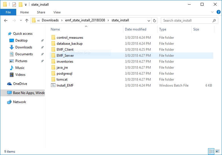
Figure 2.2 lists the batch file and the folders that are located in the install zip file; these are described below the figure.
Go to the java_jre directory and double click the executable file, jre-8u161-windows-x64.exe. (If you have a 32-bit computer, run the executable jre-8u161-windows-i586.exe.)
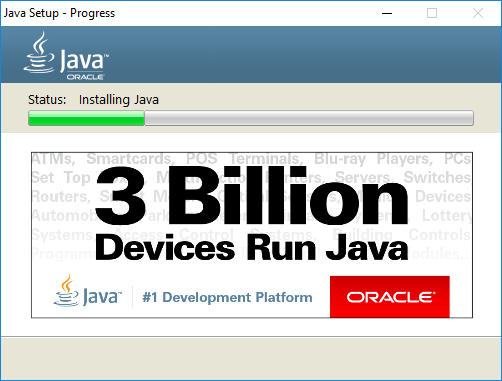
Follow the installation steps as illustrated in the figures: 2.3, 2.4, 2.5.
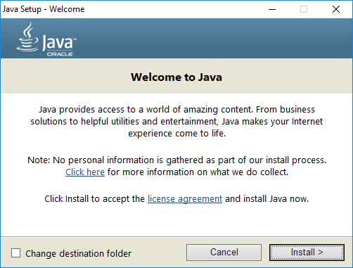
Click Install to accept the license agreement and start the installation process.
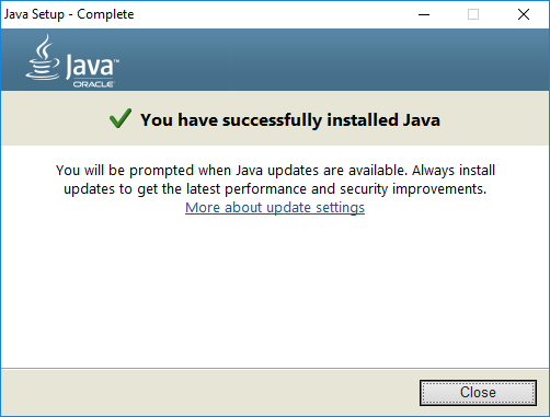
Click Close to finalize the installation process.
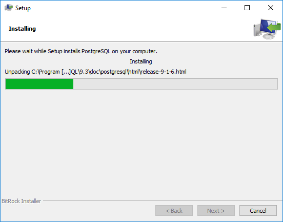
Go to the postgresql directory and double click the executable file, postgresql-9.3.9-3-windows-x64.exe. (On a 32-bit machine, run postgresql-9.3.9-3-windows.exe.)
During the installation process, you’ll be prompted to enter a database superuser password. Set a password, e.g., postgres, and take note of it for a later step of the installation process.
Follow the installation steps as illustrated in the figures: 2.6, 2.7, 2.8, 2.9, 2.10, 2.11, 2.12, 2.13, 2.14.
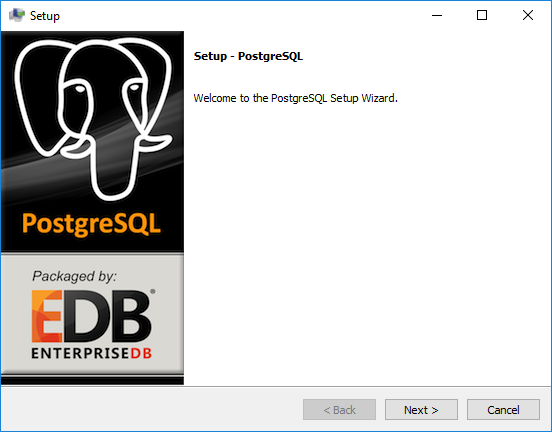
Click Next to begin the installation process.
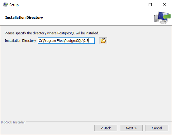
The default directory location is sufficient, click Next to continue to the next step. Remember this directory for later use in the installation process.
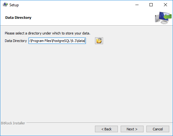
The default location is sufficient, click Next to continue to the next step.
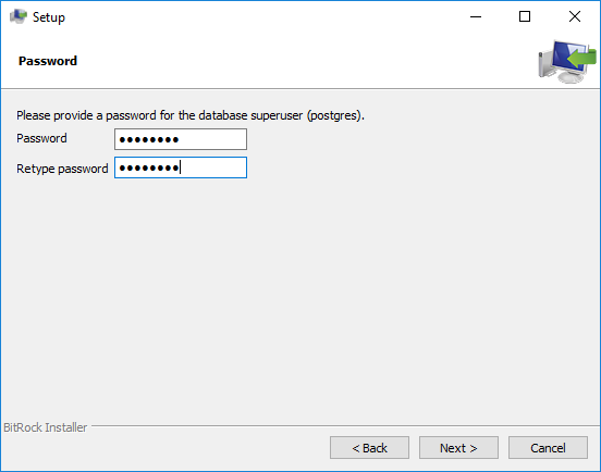
For this step, make sure you use the password that you set earlier in the installation, e.g., postgres. This password is also expected during a later step when installing the CoST database.
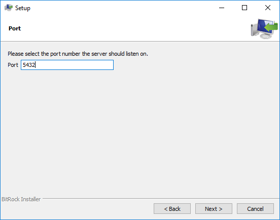
The default Port is sufficient, click Next to continue to the next step.
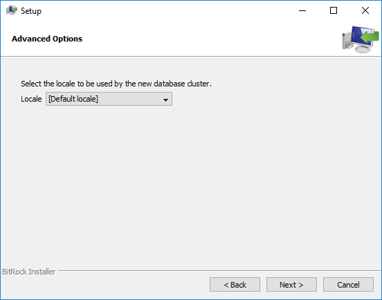
The default Locale is sufficient, click Next to continue to the next step.
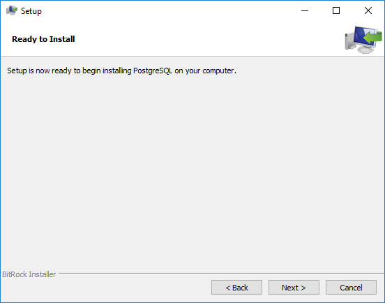
Click Next to install the PostgreSQL database server.
Click Next to finalize the PostgreSQL installation.
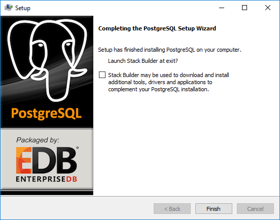
When you reach the end, uncheck the Launch Stack Builder option and click Finish.
The PostgreSQL database is now installed and ready for the CoST system database. This database will be installed in a later step.
Go to the tomcat directory and find the executable file, apache-tomcat-8.5.28.exe. Double click the file to install Tomcat. Follow the installation steps as illustrated in the figures: 2.15, 2.16, 2.17, 2.18, 2.19, 2.20, 2.21, 2.22.
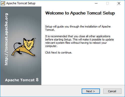
Click Next to begin the installation process.
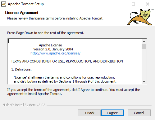
Click I Agree to continue to the next step.
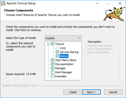
Expand the Tomcat option and check the Service Startup and Native components and then click Next. Note that the required Service Startup option ensures that the application server is available on startup when the machine is rebooted.
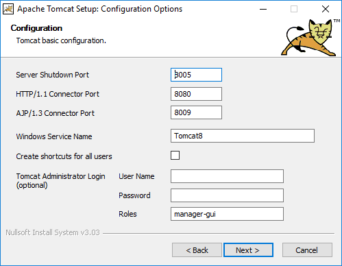
The default settings are sufficient, click Next to continue to the next step.
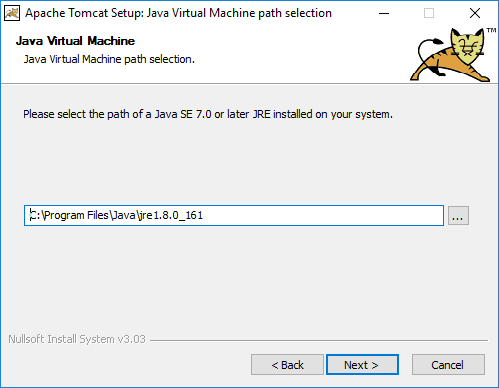
The default location is sufficient, click Next to continue to the next step.
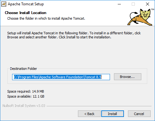
The default location is sufficient, click Install to install the Tomcat web server. Remember this folder for use in a later step of the installation process.
Once the program files have been installed click Next to finalize installation process.
When you reach the end, uncheck the box Show Readme and click Finish. The Tomcat application server is now installed and ready for the CoST system application. This CoST application will be installed in the next step.
Go to the root installation directory where the CoST/EMF zip file was installed and find the Install_EMF.bat executable file. Edit the bat file and change the following variables to match your computer’s settings:
SET EMF_CLIENT_DIRECTORY=C:\Users\Public\EMF
SET EMF_DATA_DIRECTORY=C:\Users\Public\EMF_Data
SET POSTGRESDIR=C:\Program Files\PostgreSQL\9.3
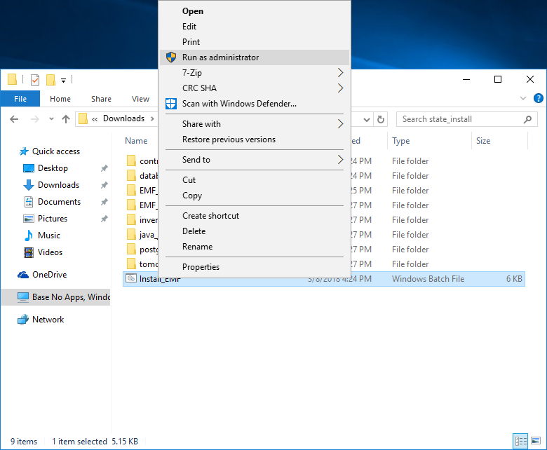
SET TOMCAT_DIR=C:\Program Files\Apache Software Foundation\Tomcat 8.5EMF_CLIENT_DIRECTORY sets the location where the EMF client application will be installed. This is the location where you will find the CoST executable.EMF_DATA_DIRECTORY sets the location where the EMF data files (e.g., inventories and control measure import files) will be installed.POSTGRESDIR sets the location where the PostgreSQL application is installed.TOMCAT_DIR sets the location where the Tomcat application is installed.Save your changes (if any), and exit the editor. Right-click the file Install_EMF.bat and select “Run as administrator” to start the CoST/EMF server installation (Figure 2.23).
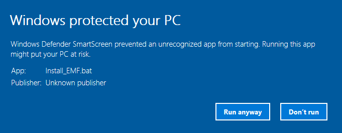
You may see a pop-up from Windows Defender, preventing an unrecognized app from starting (Figure 2.24).
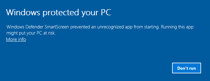
Click the link labeled “More info”, confirm the app listed is Install_EMF.bat, then click “Run anyway” (Figure 2.25).
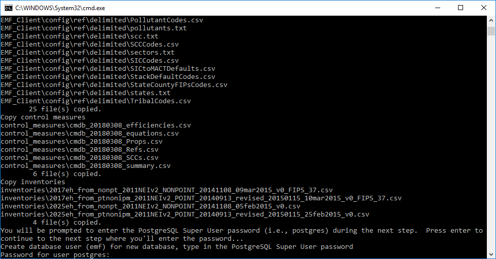
Note: This installation process can take around 30-40 minutes to finish. During the installation process, you will be prompted once (see Figure 2.26) to enter the PostgreSQL superuser password, e.g., postgres.
After the server installer completes, go to the directory containing the EMF client application; this was specified in the Install_EMF.bat file via the EMF_CLIENT_DIRECTORY variable (the default location is C:\Users\Public\EMF). Edit the EMFClient.bat batch file to match your computer’s settings:
set EMF_HOME=C:\Users\Public\EMF
set JAVA_EXE=C:\Program Files\Java\jre1.8.0_161\bin\java
EMF_HOME sets the location of EMF client application (set to be the same as EMF_CLIENT_DIRECTORY from the server installer above)JAVA_EXE sets the location of Java runtime application (note that the directory is C:\Program Files\Java\jre1.8.0_161\bin and java is the Java runtime application)Save and exit from the file EMFClient.bat.
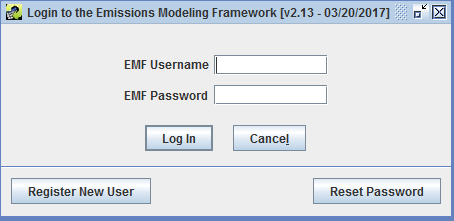
The CoST application can now be run by going to the EMF client directory and locating the EMFClient.bat file. Double click this file to start the EMF client. If Windows Defender prevents the app from starting, click the “More info” link, confirm the app listed is EMFClient.bat, then click “Run anyway”. If the configuration was specified properly and the server is running, you should see the EMF Login window (Figure 2.27).
If you have never used the EMF before, click the Register New User button. You will then see the following window (Figure 2.28):
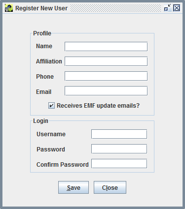
In the Register New User window, fill in your full name, affiliation, phone number, and email address. You may then select a username with at least three characters and enter a password with at least 8 characters and at least one digit and then click OK. Once your account has been created, the EMF main window should appear (see below).
If have logged into the EMF previously, enter your EMF username and password in the Login to the Emissions Modeling Framework window and click Log In.
Note: The administrator EMF login name is admin, with a password admin12345.
After successfully logging into CoST the main EMF window (Figure 2.29) will display.
The CMDB includes all of the emissions control technology information, emissions reductions, and associated costs used by the EPA for developing emissions control strategies for stationary sources. The latest CMDB is available from the EPA CoST Website.
The CoST/EMF installation package includes the latest version of the CMDB. The instructions here are provided to guide the upgrade of an existing EMF installation with a new version of the CMDB.
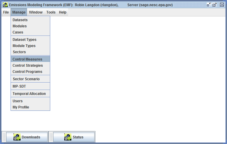
To install the CMDB in the EMF, first download the latest CMDB CSVs file from the EPA website. You must login to the EMF Client as Administrator to add to the CMDB to the CoST PostgreSQL database. After logging in as administrator select Control Measures from the Manage drop down menu at the top of the EMF Client window (Figure 2.30):
Click the Import button to see the Import Control Measures screen (Figure 2.31):
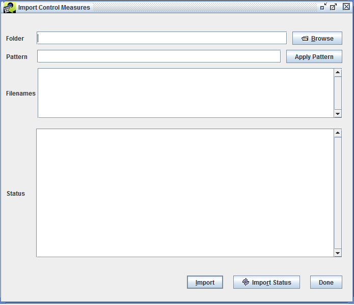
Use the Browse button to find the CMDB CSV files downloaded from the EPA website. Select the file and click OK.
Click Import to add the EPA CMDB to the CoST/EMF database.
To remove the CoST installation package, go to the root directory where the EMF/CoST Installer zip file was installed and manually remove all files and sub folders from this directory. The original zip package contains a compressed version of the installation package and can be kept for reference purposes. Removing these files and directories will free up around 1.2GB of space.
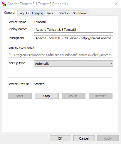
Confirm that Tomcat is running. From the Start menu, find and open the application named Monitor Tomcat (shown in Figure 2.32). Check that the Service Status is listed as Started. If Tomcat is not running, click the Start button to start the service.
Confirm that the EMF web application was installed successfully. In Windows Explorer, navigate to the Tomcat installation directory; by default, this is C:\Program Files\Apache Software Foundation\Tomcat 8.5 (Figure 2.33).
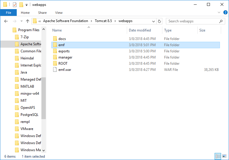
Inside the Tomcat directory, open “webapps”. You should see a file named emf.war, a directory named emf, a directory named exports, and a few other directories created by Tomcat. If you don’t see a file named emf.war, then the installation process wasn’t able to create it, most likely due to permissions issues. Make sure you run Install_EMF.bat as an administrator.
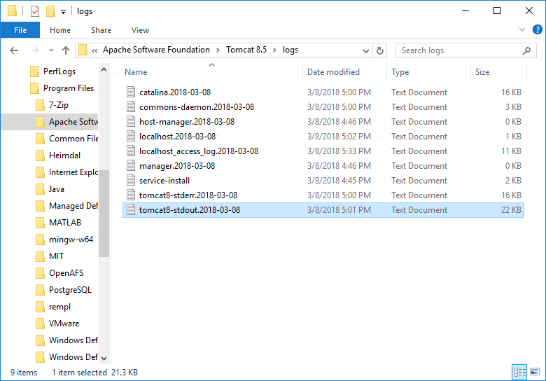
Logs for Tomcat and the EMF server can be found in the “logs” folder inside the Tomcat installation directory (e.g. C:\Program Files\Apache Software Foundation\Tomcat 8.5) (Figure 2.34). The file tomcat8-stdout.[date].log contains the console output from running the EMF server.
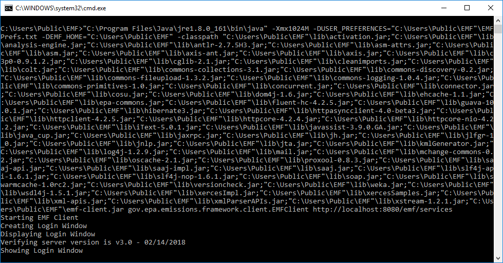
When running the EMF client, a command prompt window shows any errors or messages. A normal startup of the EMF client is shown in Figure 2.35:
This chapter demonstrates the features of the CoST Control Measure Manager. The initial CoST installation includes area- and stationary-source control measures. The pre-loaded measures can be used directly for CoST control strategy runs, the measures are editable through the CoST/EMF client, and new measures may be imported through the client. Control measures store information about control technologies and practices that are available to reduce emissions, the source categories to which they apply, the expected control efficiencies, and their estimated costs.
The Control Measure Manager allows control measure data to be entered, viewed, and edited. The data that are accessible through the Control Measure Manager are stored in the CoST Control Measures Database (CMDB). The CMDB is stored as a set of tables within the EMF database. Control measures can also be imported from files that are provided in a specific CSV format and exported to that same format. In CoST, the control measures are stored separately from the emissions inventory data and are matched with the emissions sources using a list of Source Classification Codes (SCCs) that are specified for each control measure.
The Control Measure Manager has the following major features:
In this chapter, you will learn how to:
This chapter is presented as a series of steps in a tutorial format.
Begin by opening the Control Measure Manager and exploring the buttons and menus in the upper portion of the window.
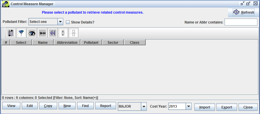
Step 1-1: Open Control Measure Manager. To open the Control Measure Manager, choose Control Measures from the Manage drop down menu on the EMF main window see Figure 2.29. The Control Measure Manager window will appear 3.1. When the window first appears, it will be empty. Notice that the window appears within the EMF main window.
Notice the different parts of the Control Measure Manager window. There is a Pollutant Filter drop down menu at the top, a Show Details checkbox, a Refresh button, and a Name or Abbr contains dialog box. Below those buttons is a toolbar with buttons that operate on the data shown in the table below the toolbar, which by default is empty. There is another set of buttons and pull-down menus below the table. The functions of all of these buttons are discussed below.
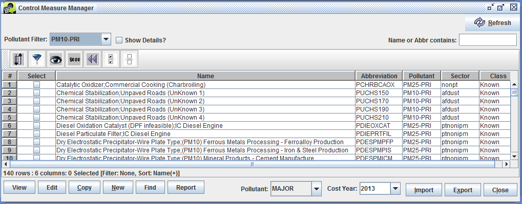
Step 1-2: Display Control Measures. To display control measures from the CMDB in the Control Measure Manager window, select a pollutant from the Pollutant Filter pull-down menu at the upper left corner of the Control Measure Manager. For this example, use the scroll bar to find and select PM10-PRI. Information about any control measures that control the selected pollutant will appear in the Control Measure Manager window (Figure 3.3). The control measure Name, Abbreviation, Pollutant, Sector, and Class are shown in the window. Note that name of each control measure must be unique within the database, and that the control measures appear in a table in which the data can be sorted by clicking on the row headers.
The control measure abbreviation is a set of characters that is a short-hand for the control measure. Typically, the abbreviation should express the name of the control measure in an abbreviated form such that if someone is familiar with the abbreviation conventions, the person might be able to infer the name of the measure. Typically the first character of the measure denotes the major pollutant (e.g., ‘P’ for PM controls, ‘N’ for NOx controls, ‘S’ for SO2 controls). The next few characters usually denote the control technology (e.g., ‘ESP’ for Electrostatic Precipitator, ‘FFM’ for fabric filter mechanical shaker). Abbreviations must be unique within the database (i.e., no two control measures can use the same abbreviation).
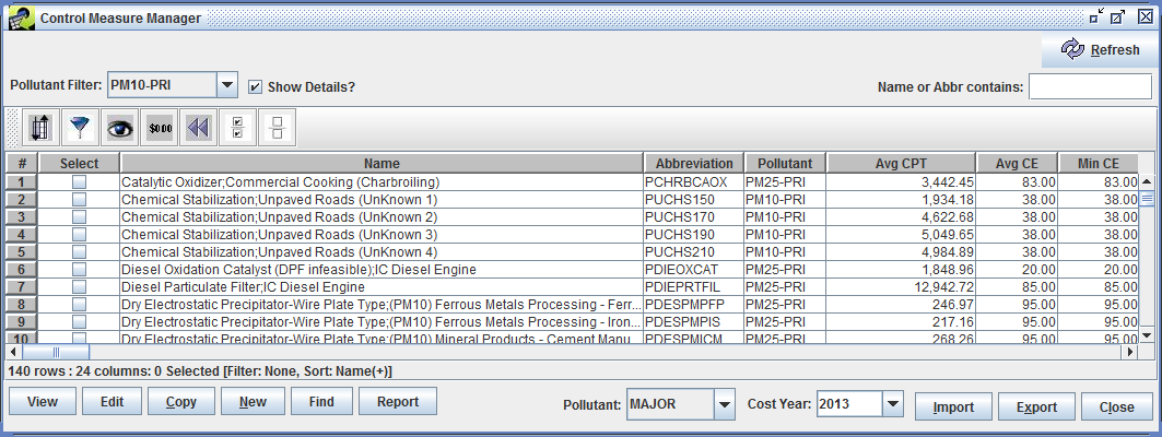
Step 1-3: Show Details of Control Measures. To see more information about the measures, check the Show Details checkbox - additional columns will appear on the right of the table. An example is shown in Figure 3.4.
Step 1-4: Configure the Control Measure Window. To better see the additional columns, you can make the Name column narrower by positioning your mouse on the line between Name and Abbreviation on the table header; this will cause a special mouse pointer with arrows to appear and you can then use the mouse to drag the column edge to resize the column width.
Step 1-5: Examine Control Measure Details. Scroll to the right to examine the detail columns that are available in the Control Measure Manager. Note that you may move the columns around by grabbing the column’s header with your mouse and dragging them. You may also change their widths as desired. You can also resize the Control Measure Manager window within the EMF Main Window as desired, such as to make the entire window wider so that you can see more columns.
Step 1-6: View Measure Name. After you scroll to the right in the window, if you hover your mouse over one of the columns other than Name, you will see that the name of the measure corresponding to the row you are on will appear briefly as a “tooltip”. This is so that you can tell what the name of the measure is even if it has scrolled off the window.
The columns shown on the Control Measure Manager with brief descriptions are shown in Table 3.1. The control measures table supports sorting and filtering the data. Tables of this same type are used many places throughout CoST and the EMF.
| Column Name | Description |
|---|---|
| Select | This column will allow the user to view, edit, or copy the measure by clicking the corresponding button at the bottom of the manager window. These features will be discussed later in the training. |
| Name | A unique name for the measure. |
| Abbreviation | A unique abbreviation for the measure. |
| Pollutant | A pollutant (e.g., NOx, PM10-PRI) that the measure might control. Note that any pollutant-specific information in the row is for this pollutant. |
| Avg, Min, and Max CE | Average, minimum, and maximum control efficiencies for the specified pollutant, aggregated across all locales, effective dates, and source sizes. |
| Avg, Min, and Max CPT | Average, minimum, and maximum cost per ton for the specified pollutant aggregated across all locales, effective dates, and source sizes. |
| Avg Rule Eff. | Average rule effectiveness aggregated across all efficiency records for the specified pollutant. |
| Avg Rule Pen. | Average rule penetration aggregated across all efficiency records for the specified pollutant. |
| Control Technology | The control technology that is used for the measure (e.g., Low NOx burner, Onroad Retrofit). |
| Source Group | The group of sources to which the measure applies (e.g., Fabricated Metal Products - Welding). |
| Equipment Life | Expected lifetime (in years) of the equipment used for the measure. |
| Sectors | An emissions inventory sector or set of the EPA’s emissions inventory sectors to which the measure applies (e.g., ptipm, afdust, nonpoint). A sector represents a broad group of similar emissions sources. |
| Class | The class of the measure. Options are Known (i.e., already in use), Emerging (i.e., realistic, but in an experimental phase), and Hypothetical (i.e., the specified data are hypothetical). |
| Eq Type | The type of COST equation to use |
| Last Modified Time | The date and time for which the information about the measure was last modified in the editor or imported from a file. |
| Last Modified By | The last user to modify the measure. |
| Date Reviewed | The date on which the data for the measure were last reviewed. |
| Creator | The user that created the measure (either from the import process or by adding it via the “New” button). |
| Data Source | A description of the sources or references from which the values were derived. Temporarily, this is a list of numbers that correspond to references listed in the References Sheet from when the control measures were imported. |
| Description | A textual description of the applicability of the measure and any other relevant information. |
Step 1-7: Sort Control Measures. To sort based on data in one of the columns, click on the column header. For example, to sort based on the average control efficiency of the measure click on the column header for the “Avg CE” column. The table will now be sorted by the values of “Avg CE” in descending order. Notice that information about the currently specified sort is reflected in the line just below the table.
Step 1-8: Reverse Sort. Click on the header of the “Avg CE” column a second time, the sort order will be reversed.
Step 1-9: Multi-Column Sort. To perform a multicolumn sort, click the sort button  and then click
 Add to add an additional column to sort by (e.g., Name). Notice that you can control whether the sort is Ascending and whether it is Case Sensitive. Click OK once you have made your selection. The data should now be sorted according to the column(s) you specified.
Step 1-10: Apply Filters to Control Measure Table. To use a filter to limit the measures shown, click the button on the toolbar that looks like a filter  . When you do this the “Filter Rows” dialog appears (Figure 3.5).
Add Criteria.Operation to see the available operations and, if desired, select an operation (contains is the default).Value cell (e.g., Scrubber). Note that the filter values are case-sensitive (e.g., Measure names containing “scrubber” will not match a filter value of “Scrubber”).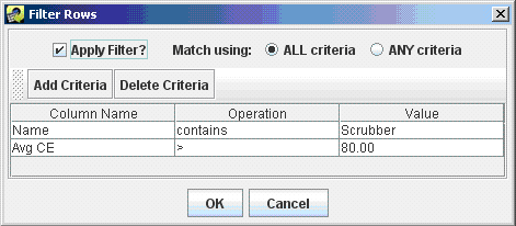
To add a second criterion click Add Criteria again on the Filter Rows dialog (e.g., enter ‘Avg CE > 80’). Note that if Match using is set to ALL criteria then only rows that match all the specified criteria will be shown in the table after you click OK. If Match using is set to ANY criteria, then rows will be shown in the table if they meet any of the criteria that are listed.
Click OK to close the Filter Rows dialog and to apply the selected filter. Figure 3.6 shows the table that results from the selections shown in Figure 3.5. Notice that the currently applied filter is reflected in the line under the horizontal scrollbar of the table.
Open the filter dialog again by clicking the Filter rows button. Set Match using to ANY criteria and then click OK to see what effect it has on the measures shown. Hint: you should see more measures displayed than when Match using is set to ALL criteria.
Step 1-11: Remove Filters from the Control Measures Table. Open the filter dialog again by clicking the Filter rows button. Remove one of criteria by clicking somewhere in one of the rows shown on the Filter Dialog and then clicking Delete Criteria. Now click OK to have the less stringent filter take effect.
Step 1-12: Select and Unselect Control Measures. To select all of the control measures that meet your filter criteria, click the Select All button on the toolbar  . You will see that the checkboxes in the
 Select column are now all filled with checks. You may select or deselect individual measures by clicking their checkboxes in the Select column. In the next subsection, we will discuss operations that can be performed on selected measures, such as viewing them and exporting their data.
To unselect all of the measures, click the Clear all the selections button ![]() and you will see that all of the checks in the
and you will see that all of the checks in the Select column are now removed.
Step 1-13: Show/Hide Columns. To hide some of the columns that are shown in the table, click the Show/Hide columns button  . On the Show/Hide Columns dialog that appears (similar to the one shown in Figure 3.7, uncheck some of the checkboxes in the
 Show? column and then click OK. The columns you unchecked will no longer display in the control measures table.
Click the Show/Hide columns button again and scroll down through the list of columns at the top of the dialog to see others that are farther down the list. To select multiple columns to show or hide, click on the first column name of interest, hold down the shift key, then click a second column name to select the intervening columns, and then click the Show button or the Hide button to either show or hide those columns.
To select columns that are not next to each other, hold down the control key and click on the columns that you want to select; when you are finished selecting click Show or Hide. The remaining buttons on the dialog are not used frequently: (a) Invert will invert the selection of highlighted columns. (b) The Add Criteria/Delete Criteria Filter section at the bottom can be used to locate columns when there are hundreds of column names, but there are no tables that large used in CoST.
Step 1-14: Format Columns. Click the Format Columns button,  , to open the Format Columns dialog and examine the options for controlling how data in the table are shown. For example, check the checkboxes in the
 Format? column for one or more of the column names “Avg CE”, “Min CE”, and “Max CE” (note that you may first need to unhide the columns if you hid them in the previous step). Because these columns are all numeric, some controls used to format numbers will appear in the lower right corner.
Change the Font to Arial, the Style to Bold, the Size to 14, the Horizontal Alignment to Left, the Text Color to blue, the Column Width to 6, the number of Decimal Places to 0, and select Significant Digits. Once these selections have been made, the dialog should look similar to the one in Figure 3.8. Click OK after making these selections to apply the formatting to the Control Measures table. The columns selected for formatting will have the attributes specified on the Format Columns dialog. In practice, this dialog is not used very often, but it can be particularly helpful to format numeric data by changing the number of decimal places or the number of significant digits shown.
Step 1-15: Reset Control Measures Table. To remove sort criteria, row and column filters, and formatting, click the Reset button  in the Control Measure Manager window.
Step 1-16: Mouse Hover Tooltip. If you are unsure of what a button does when using CoST, place your cursor over the button and wait; in many cases, a small piece of text called a “tooltip” will appear. For example, place your cursor over one of the buttons on the Control Measure Manager window and hold it still. You will see a tooltip describing what the button does. Many of the buttons and fields used in CoST have tooltips to clarify what they do or what type of data should be entered.
Step 1-17: Update Control Measures List. If you wish to retrieve an updated set of control measures data from the CoST server, click the Refresh button  at the upper right portion of the Control Measure Manager. Note that this will also reset any special formatting that you have specified, but any sort and filter settings will be preserved.
In this section you will learn about viewing the detailed data for a control measure.
Step 2-1: Select a Control Measure. Select the control measure for which to view the underlying data. For example, in the Control Measure Manager, set the Pollutant Filter to PM10-PRI, and then in the table locate the Control Measure with the Name “Dry Electrostatic Precipitator-Wire Plate Type;(PM10-PRI) Municipal Waste Incineration” (Abbreviation = PDESPMUWI).
Hint: Typing the abbreviation into the Name or Abbr contains box will display the measure directly.
Step 2-2: View Control Measure Data. Click the checkbox in the Select column next to the measure and click View. The View Control Measure window will appear as shown in Figure 3.9. There are several tabs available on the window; the Summary tab will be shown by default.
Step 2-3: Examine Control Measure Summary. The Summary tab of the View Control Measure window contains high-level summary information about the measure. Table 3.2 shows brief descriptions of the fields on this tab.
| Component | Description |
|---|---|
| Name | A unique name that typically includes both the control technology used and the group of sources to which the measure applies. |
| Description | A description of the applicability of the measure and any other relevant information. |
| Abbreviation | A multi-character unique abbreviation that is used to assign the control measure to sources in the inventory. Ideally, the abbreviation should be somewhat readable so that the user has some idea of what type of measure it is from reading the abbreviation (e.g., the DESP in PDESPIBCL is short for ‘Dry Electrostatic Precipitator, the IB is short for ’Industrial Boiler’, and the CL is short for ‘Coal’). |
| Creator | The name of the user who imported or created the measure. |
| Last Modified Time | The date and time on which the information about the measure was last modified in the editor or imported from a file. |
| Last Modified By | The last user to modify the measure. |
| Major Pollutant | The pollutant most controlled by the measure. This is used to group the measures only, and has no impact on how the measure is assigned to sources. |
| Control Technology | The control technology that is used for the measure (e.g., Low NOx burner). You can type a new entry into this field and then choose it from the pull-down menu in the future. |
| Source Group | The group of sources to which the measure applies (e.g., Fabricated Metal Products - Welding). You can type a new entry into this field and then choose it from the pull-down menu in the future. |
| NEI Device Code | The numeric code used in the NEI to indicate that the measure has been applied to a source. A cross-reference table to match the control measure abbreviations and NEI Device Codes to one another may be created. |
| Class | The class of the measure. Options are Known (i.e., already in use), Emerging (i.e., realistic, but in an experimental phase), Hypothetical (i.e., the specified data are hypothetical), and Temporary (i.e., the specified data are temporary and should be used only for testing purposes). |
| Equipment Life | The expected life of the control measure equipment, in years. |
| Date Reviewed | The date on which the data for the measure were last reviewed. |
| Sectors | An emissions inventory sector or set of emissions inventory sectors to which the measure applies. A sector represents a broad group of similar emissions sources. |
| Months | The month(s) of the year to which the control measure is applicable. This is either “All Months” or a list of individual months (e.g., March, April, and May for measures applicable only in spring months). |
When viewing a control measure (as opposed to editing a control measure), you cannot make changes to any of the selections. However, you can review the available selections for some fields. Use the pull-down menus next to the fields Major Pollutant, Control Technology, Source Group, and Class to see the available options for each of these fields. Note that if you make a selection that differs from the original value on one of these menus, the new value will not be saved when you close the window because you are only viewing the measure data.
Step 2-4: Examine Control Measure Efficiencies. Click on the Efficiencies tab in the View Control Measure Window to see the data that are available from this tab. You will see a table with many columns. Each row in the table corresponds to a different “efficiency record” in the database. An efficiency record contains cost and control efficiency information about the control measure. In the example shown in Figure 3.10, notice that the Control Efficiency and cost per ton data (CPT) vary by pollutant. Scroll to the right in the table to see some of the other columns that are not immediately visible.
If the cost or control efficiency varies over region or time, it is possible to specify different records in the table for each Locale (i.e., state or county) or for each Effective Date if the measure will be “phased in” over time. Different efficiency records can also be entered to account for different source sizes using the Min Emis and Max Emis columns.
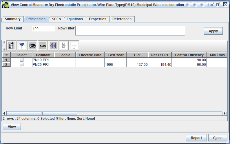
The Row Limit and Row Filter fields are helpful when there are hundreds of efficiency records (e.g., some data may be county specific and available for multiple pollutants). The Row Limit is the maximum number of records that will be displayed on the page. For example, if there were several hundred records, it could take a long time to transfer all of those data from the server, so by default only 100 records will be transferred if the Row Limit is set to 100.
Step 2-5: Apply a Row Filter to Control Measure Efficiencies. To apply a Row Filter to the control efficiencies, enter Pollutant='PM10-PRI' into the text field and then click Apply to display only the record for PM10-PRI. The Row Filter follows the syntax of a Structured Query Language (SQL) ‘WHERE’ clause. Note that the filter may not seem necessary in this particular example that only has a few records, but if this measure had entries for every county and pollutant, as do some mobile measures, then the filter is useful for limiting the number records displayed. If desired, you may try some other filters with this measure, such as:
Pollutant LIKE 'PM%'
Pollutant = 'PM10-PRI'
Control Efficiency > 95
Here are some examples of other types of filters that illustrate other aspects of the syntax, although they may not all be applicable to this particular measure:
Pollutant != 'PM10-PRI'
Locale LIKE '37%'
Pollutant IN ('CO', 'VOC', 'PM10-PRI')
Step 2-6: View an Efficiency Record in a Separate Window. To see the data for an efficiency record in a separate window, check the checkbox in the Select row for the PM25-PRI efficiency record, and click View. A View Efficiency Record window will appear as shown in Figure 3.11. The fields of the efficiency record are shown in Table 3.3.
Notice that most of the fields in Figure 3.11 are set using text fields. The Ref Yr Cost Per Ton Reduced is shown with a label because this value is automatically computed for the reference year (currently 2013) according to the cost year and the specified Cost Per Ton Reduced. Note that the cost per ton reduced should take into account the specified rule effectiveness and rule penetration, which can ‘dilute’ the effectiveness of the control measure, but are not taken into account when the Ref Yr Cost Per Ton Reduced is computed. Other fields that are labels are Last Modified By and Last Modified Time. These fields are automatically updated and tracked by CoST when someone edits the efficiency record, although editing is done from the Edit Efficiency Record window instead of the View Efficiency Record window.
Note: The efficiency records must be unique according to the contents of the following fields: Pollutant, Locale, Effective Date, Existing Measure Abbreviation, Existing NEI Device Code, Minimum Emissions, Maximum Emissions, Minimum Capacity, and Maximum Capacity. This means that two records cannot have the same values for all of these fields.
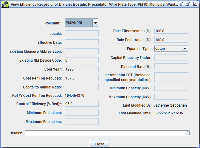
| Component | Description |
|---|---|
| Pollutant | The pollutant for which this record applies (emissions are either decreased or increased). An asterisk appears beside this field because a value for it must be specified. |
| Locale | A two-digit Federal Information Processing Standards (FIPS) state code, or a five-digit FIPS county code, to denote that the information on the row is relevant only for a particular state or county. If left blank, it is assumed to apply to all states and counties. |
| Effective Date | The month, day, and year on which the record becomes effective. The system will find the record with the closest effective date that is less than or equal to the date of the analysis. If this is left blank, the record is assumed to apply to any date. |
| Existing Measure Abbreviation | This field should be populated when the data on the row are provided, assuming that a control measure has already been applied to the source. The contents of the field should be the control measure abbreviation that corresponds to the existing measure. The reason for this field is that the efficiency of and cost of applying the measure may vary when there is already a control measure installed on a source. |
| Existing NEI Device Code | This is used in conjunction with Existing Measure and should specify the device code used in the NEI that corresponds to the currently installed device. |
| Cost Year | The year for which the cost data are provided. |
| Cost per Ton Reduced | The cost to reduce each ton of the specified pollutant. |
| Capital to Annual Ratio | The ratio of capital costs to annual costs. |
| Ref Yr Cost per Ton Reduced | The cost per ton to reduce the pollutant in 2013 dollars. |
| Control Efficiency | The [median] control efficiency (in units of percent reduction) that is achieved when the measure is applied to the source, exclusive of rule effectiveness and rule penetration. An asterisk is shown next to the field because a value for the field is required, whereas other fields are optional. Eventually, statistical distributions for percent reduction may be provided to facilitate uncertainty analysis. Note that there are sometimes disbenefits for certain pollutants as a result of the control device, so control efficiency can be negative to indicate that the amount of a pollutant actually increased. |
| Minimum Emissions | The lower limit of emissions from the inventory required for the control measure to be applied. |
| Maximum Emissions | The upper limit of emissions from the inventory for the control measure to be applied. |
| Rule Effectiveness | The ability of a regulatory program to achieve all the emissions reductions that could have been achieved by full compliance with the applicable regulations at all sources at all times. A rule effectiveness of 100% means that all sources are fully complying at all times. Rule effectiveness can sometimes vary by locale. |
| Rule Penetration | The percent of sources that are required to implement the control measure. Rule penetration might vary over time as a new rule is “phased in” gradually, and can sometimes vary by locale. |
| Equation Type | Unused |
| Capital Recovery Factor | Unused |
| Interest Rate (%) | Unused |
| Incremental CPT | Unused |
| Minimum Capacity (MW) | The minimum capacity for the control measure (megawatts). |
| Maximum Capacity (MW) | The maximum capacity for the control measure (megawatts). |
| Last Modified By | The last user to modify the efficiency record. |
| Last Modified Time | The last date and time a user modified the efficiency record. |
| Details | Text that specifies information about the source of data for this row or reason they were changed. |
When you are done examining the information on the View Efficiency Record Window, click Close.
Step 2-7: View the Control Measure SCCs. The inventory sources to which a control measure could be applied are listed in the SCCs tab for the control measure.
Note that while multiple SCCs can be specified for a measure, if the control efficiency or cost data differs for any of the SCCs, then a separate measure must be created to contain that data.
Click on the SCCs tab in the View Control Measure window to see the SCCs associated with the measure. An example of this tab is shown in Figure 3.12. The selected control measure is applicable only to SCCs listed on this tab.
Note that CoST currently does not support wildcards in the SCC list for a control measure. There is no expanding of SCC codes ending in zeros; therefore each applicable SCC must be explicitly listed on this tab. You may sort and filter the SCCs in the table to get a better idea of what SCCs are associated with the measure.
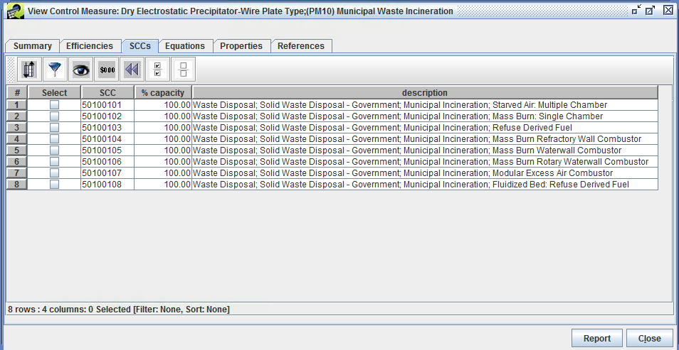
Do not click Close after examining the SCC list as this will close the View Control Measure window, which we will use for the next step.
As an alternative to using a simple ‘cost per ton of pollutant reduced’ value to compute the cost of a control measure, an engineering cost equation can be specified. The cost equation will then be used to associate emissions control costs with a particular pollutant. The equation must be selected from a list of pre-specified equation types. The cost will be computed using the form of the equation specified on the equations tab, source-independent variables listed in the equations tab, and source-dependent variables from the emissions inventory (e.g., stack flow rate). Currently, only a single equation can be specified for any given measure.
Step 2-8: View the Control Measure Equations. Click on the Equations tab on the View Control Measure window to see information associated with the cost equations for the selected measure. An example of this tab is shown in Figure 3.13. If the measure does not use a cost equation, this tab will be blank. The table at the bottom of the Equations tab shows the Equation Type (the same type is repeated in every row), in addition to the Variable Name and Value for that variable. The fields of the Equations tab are shown in Table 3.4.
Each type of equation uses a different set of variables. CoST supports fourteen different types of cost equations. Additional types of equations may be added in the future. For more information on the equations and their input variables, see the Documentation of Cost Equations in the EPA’s Control Strategy Tool (CoST). The appropriate form of the equation will be used in conjunction with the specified values to compute the total cost of applying the measure to the source for the specified pollutant and cost year.
Do not click Close after examining the Equations tab as this will close the View Control Measure window, which we will use for the next step.
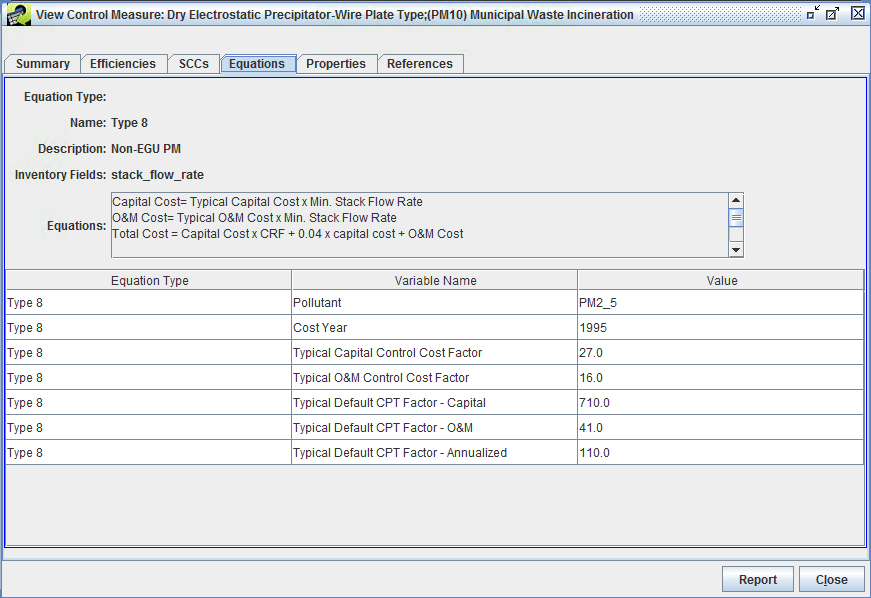
| Component | Description |
|---|---|
| Name | The name of the engineering cost equation type (e.g., Type 8). |
| Description | The description of the engineering cost equation type (e.g., Non-EGU PM Cost Equation). |
| Inventory Fields | The input parameters to the cost equations found in the inventory (e.g., stack velocity and temperature or design capacity). |
| Equations | The cost equation definitions. |
Step 2-9: View the Control Measure Properties. Click on the Properties tab on the View Control Measure window to see the data that are available from this tab. Each row in the Properties tab corresponds to a different “property record” in the database. A property record allows for generic information to be stored about the control measures (e.g., metadata). The control measures example in Figure 3.14 shows property information that happened to be archived from the AirControlNET software when the measures were transferred into the CMDB.
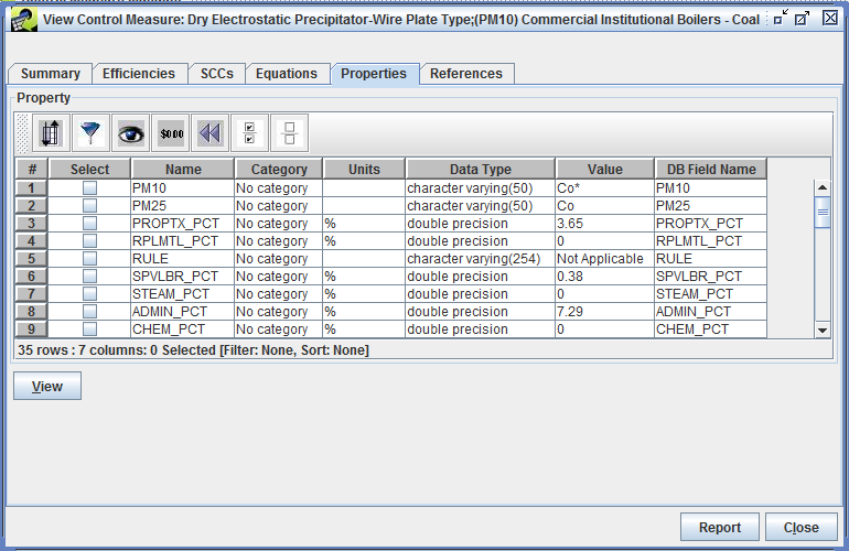
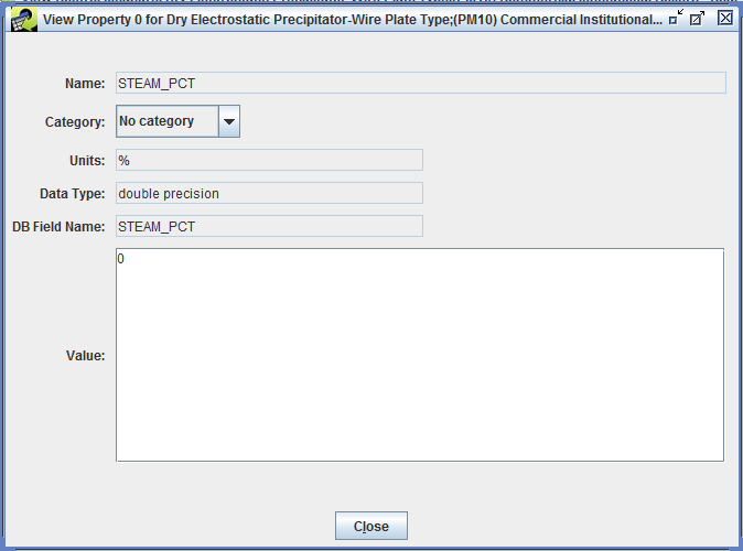
Step 2-10: View a Properties Record in a Separate Window. To see the data for a property record in a separate window, check a checkbox in the Select column and click View. For example, select the STEAM_PCT property record and click View. Figure 3.15 shows the View Property Record window that will appear. The fields of the property record are shown in Table 3.5.
Notice that most of the fields in Figure 3.15 are set using text fields. The Category is a free-form drop down, where an existing category could be used or a new one could be used by typing in the new category.
Do not click Close after examining the Properties tab as this will close the View Control Measure window, which we will use for the next step.
| Component | Description |
|---|---|
| Name | The name of the property. |
| Category | The category for the property (e.g., AirControlNET Properties, Cost Properties, or Control Efficiency Properties). |
| Units | The units for the property (e.g., % for percentage). |
| Data Type | If applicable, this defines the data type of the property (e.g., double precision/float for numeric values, or a varchar/string for textual information). |
| DB Field Name | If specified, this is a placeholder to help identify the database field name from the particular data source reference that supplied the property information (e.g., an ancillary dataset has a steam percentage stored in the STEAM_PCT table field/column). |
| Value | The value of the property. |
Step 2-11: View the Control Measure References. Click on the References tab of the View Control Measure window to see the report and literature citations associated with a control measure (Figure 3.16). Each row in the table corresponds to a different “reference record” in the database. A reference record stores source and reference information for the primary information used to create a control measure.
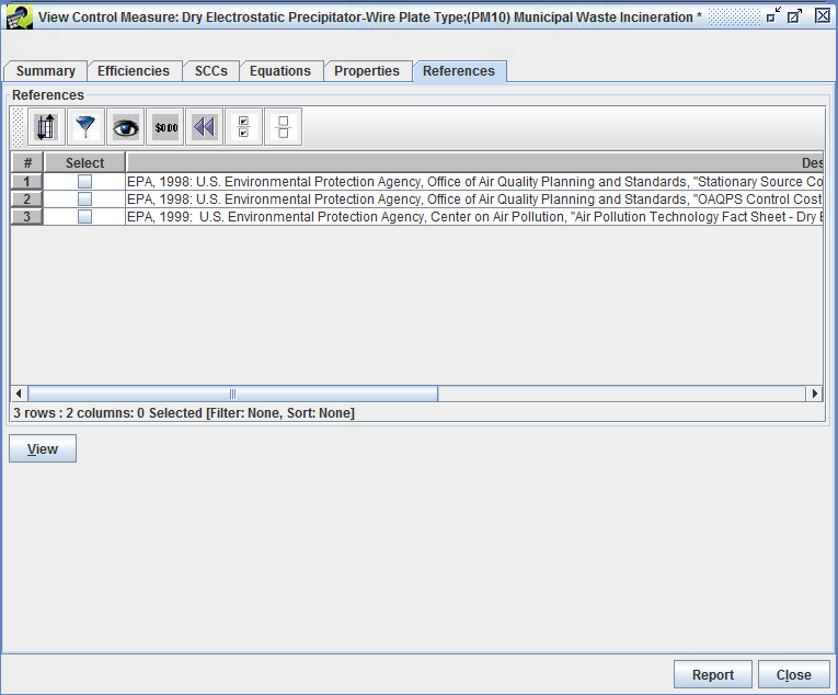
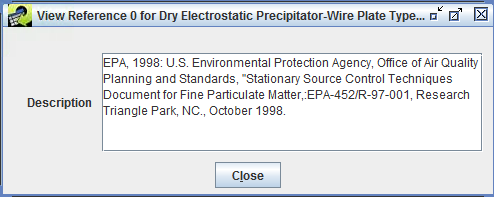
Step 2-12: View a References Record in a Separate Window. To see the data for a reference record in a separate window, check a checkbox in the Select column and click View. For example, check the checkbox for the first reference record and click View. A View Reference Record window will appear (Figure 3.17) with an editable source/reference description text field.
When you are done examining the information on the View Reference Record Window, click Close.
This concludes the exercises on examining existing control measures. Click Close to close the View Control Measure window.
One way to create a new control measure in CoST is to copy an existing control measure and then edit its data.
Step 3-1: Copy a Control Measure. To copy a control measure, first find a measure to copy. Start by clicking the Reset button on the toolbar of the Control Measure Manager to remove any previously specified filters.
Next, uncheck the Show Details button at the top of the Control Measure Manager (to speed the data transfer) and set the Pollutant Filter at the top of the Control Measure Manager to the pollutant of interest. For this example select NOx and find the measure named “Selective Non-Catalytic Reduction; ICI Boilers - Natural Gas” (Abbreviation = NSNCRIBNG). Hint: You may want to apply a filter to the manager to make it easier to find this specific measure.
Once you have found the measure to copy, check the corresponding checkbox in the Select column and then click the Copy button. CoST will create a new control measure called “Copy of [the starting measure name] [your name] [unique #]”. A unique abbreviation will also be automatically generated for the measure.
Step 3-2: View the Copied Control Measure. To see the new control measure in the Control Measure Manager, Scroll to the top of the window. If you do not see the measure, click the Refresh button at the top right of the Manager window to obtain updated data from the CoST server.
Note: If the measure named ‘Copy of Selective Non-Catalytic Reduction; ICI Boilers…’ still does not appear, a filter may be active that is preventing the measure from showing up. Remove any filters to see the newly copied measure.
View the contents of the copied measure by selecting the checkbox next to the measure and clicking the View button. The new measure will be edited in the next section.
Only control measures created by the current CoST user can be edited through the Control Measure Manager. CoST Administrators can edit all of the measures in the CMDB.
Step 4-1: Find a Control Measure to Edit. First, click the Clear all the selections button to unselect any previously selected measures ![]() . For this exercise, find the measure created using the copy button (see Copying a Control Measure) in the Control Measure Manager and check the corresponding select box in the Select column. Click
. For this exercise, find the measure created using the copy button (see Copying a Control Measure) in the Control Measure Manager and check the corresponding select box in the Select column. Click Edit to edit the data for the control measure. The Edit Control Measure window will appear Figure 3.18.

Like the View Control Measure window, the Edit Control Measure window has six tabs, and the Summary tab is shown by default. The main difference between the View and Edit windows is that the control measure contents can be changed in the Edit window, rather than just viewing the information.
Notice that most of the fields have white backgrounds, which usually indicates that the field is editable; fields that are not contained within boxes are set by the software and cannot be changed by the user. In addition, there are Add and Remove buttons for the lists of Sectors and Months.
Step 4-2: Change a Control Measure Name. The name of a control measure can be changed on the Summary tab of Edit Control Measure window. For example, you may change the part of the measure name that deals with the affected sources, such as Selective Non-Catalytic Reduction; ICI Boilers - Natural Gas and Oil. Recall that measure names must be unique.
When the measure was copied, the abbreviation was set to a number that was known to be unique so that it could be saved in the database. Replace the automatically generated Abbreviation for the new measure with something else (e.g., NSNCRIBNGO). Try to follow a similar naming convention as the other measures, but your new abbreviation must be unique in the database.
Step 4-3: Edit Other Fields in the Control Measure Summary. Edit the other Summary fields of the measure as desired. For this exercise, change the Equipment Life to 10, change the Date Reviewed to today’s date, set Class to Emerging, and make any other changes you wish, such as entering a more detailed Description.
Click the Add button under the Sectors list to add another sector for the measure. For example, from the Select Sectors dialog, choose ptipm (i.e., point sources handled by the Integrated Planning Model) and click OK. You will then see the new sector added to the list of applicable sectors. Note that the sectors listed here are informational only; they do not affect the use of the measure in control strategies in any way.
Step 4-4: Remove a Control Measure Sector. To remove a sector from a Control Measure, click on the sector in the list and click Remove and it will no longer appear on the list.
Step 4-5: Setting Months for a Control Measure. Adding and removing Months to which a control measure applies works similarly to adding and removing sectors. For this exercise, specify some particular months to which the measure should apply (e.g., March, April, and May).
Note: the feature of setting specific months for which a measure applies is effective only when applying measures to monthly emissions inventories. Specifying months in this way is not effective when applying measures to annual emissions inventories.
To set the months back to All Months, select all of the months in the Months list by clicking on the first month, scrolling to the last month in the list, and using shift-click with your mouse to select all of the months in the list. Click Remove to remove specific months and to set the measure to be applicable to all months.
Step 4-6: Discard Changes. Now that you have changed information for the measure, notice that an asterisk (*) appears after the measure name in the title for the window. This means that CoST is aware that you have made changes. If you try to Close a window on which you have made changes to the data without saving it, CoST will ask you “Would you like to discard the changes and close the current window?” If you want to discard (i.e., undo) ALL of the changes made since you started editing the measure, click Yes. If you prefer to not to close the window so that your changes stay in-tact, click No. For this exercise, click No to preserve the changes that you made.
Step 4-7: Edit Control Measure Efficiencies. Go to the Efficiencies tab of the Edit Control Measure Window Figure 3.19. The buttons on the Efficiencies tab of the Edit window are different from those on the View window. The available buttons are Add, Edit, and Remove. Notice the efficiency record for the measure shown in Figure 3.19 is for only one pollutant, and that this record can be applied only to sources emitting at least 25 tons/yr as specified in the Min Emis field.
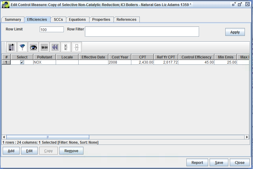
Scroll to the right to examine additional fields. Note that more of the fields are filled in for NOx than for the PM measure that you examined in Viewing Data for an Existing Control Measure. The additional data allows CoST to compute the capital and operating and maintenance (O&M) costs in addition to overall annualized costs when this measure is used in a control strategy.
To edit an efficiency record, check the checkbox in the Select column for the pollutant to edit and then click Edit. The Edit Efficiency Record window will appear Figure 3.20.
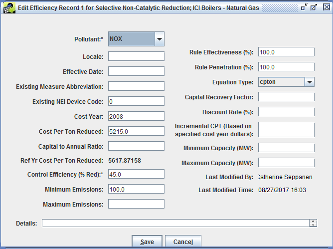
Edit the values for the efficiency record to configure the new control measure. For this exercise, set Maximum Emissions to 5000 and click Save. The value for this field is now updated in the table in the Edit Control Measure window. The measure will apply only to sources that emit between 25 and 5000 tons of NOx annually.
Step 4-8: Add a Control Measure Efficiency Record. To add a new efficiency record, click Add in the Edit Control Measure Efficiencies tab. Fill in the fields in the Add Efficiency Record window to create the new Efficiencies record. For this exercise, select CO2 as the Pollutant, set Locale to 06, set Effective Date to 01/01/2025, and set Control Efficiency (% Red) to 10. Click Save to save the new record. A new row will appear in the table on the Efficiencies tab in the Edit Control Measure window. The effect of this new record will be to include a 10% reduction to CO2 emissions for sources in California (FIPS=06) starting on 01/01/2025 when this control measure is applied.
Step 4-9: Remove a Control Measure Efficiency Record. To remove one or more efficiency records, click the corresponding checkboxes next to the record and then click Remove to remove those records. For this exercise, click the checkbox in the Select column for the CO2 record that you just added and click Remove to remove that record. When asked to confirm removal of the selected record, click Yes. The record will disappear from the Efficiencies tab.
Additive impact of multiple efficiency records. If cost per ton (CPT) values are specified for multiple efficiency records, they are additive when they are used in a control strategy. For example, if a CPT is specified for both NOx and VOC for a measure, the total cost of applying the measure is the sum of (1) the CPT for NOx times the NOx emissions reduced and (2) the CPT for VOC times the VOC emissions reduced.
Step 4-10: Edit Control Measure SCCs. Click on the SCCs tab on the Edit Control Measure window to show the SCCs for inventory sources to which the edited measure can be applied. SCCs may be added or removed for a measure from this window. An example of this tab is shown in Figure 3.21.
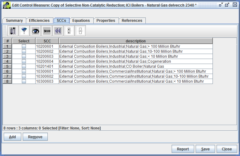
To add new SCCs, click the Add button to display the Select SCCs window (Figure 3.22). Note that there are over 11,900 possible SCCs to use for developing control measures. The number of available SCCs can be found in the lower left hand corner of the Select SCCs dialog.
To filter the SCCs for the new measure on the Select SCCs window, click the Filter Rows button on the toolbar. For this exercise, when the Filter Rows dialog that appears, click Add Criteria three times, enter the following criteria, then click OK:
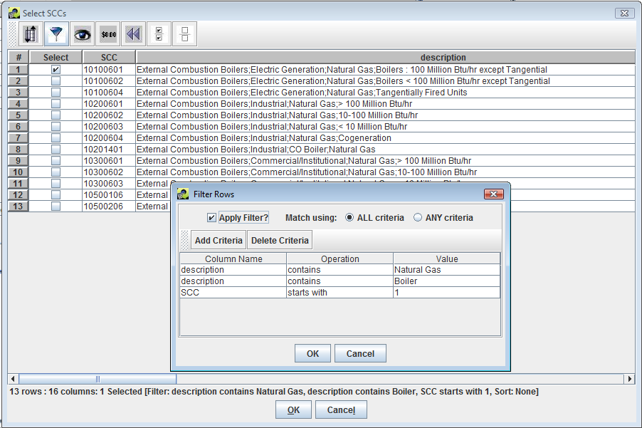
The Select SCCs window will show only the SCCs that met the above criteria, such as the 13 SCCs shown in Figure 3.22. While many of these SCCs are already associated with the measure (i.e., they are already shown on the SCCs tab of the Edit Control Measure window in Figure 3.21, a few additional SCCs (i.e., the ones starting with 101 and 105) are also relevant for this measure.
Step 4-11: Add SCCs to a Control Measure. Click the checkbox in the Select column for the SCCs to add to the measure. For this exercise, select 10100601 and then click OK. The SCC will now appear in the list of applicable SCCs for the measure in the Edit Control Measure window. Note: If you select an SCC to add that was already on the SCCs tab, it will not cause any problems and it will not add the SCC for a second time.
Tip for adding multiple of SCCs: If you need to add several SCCs and are able to specify a filter on the Select SCCs dialog box that results in only the SCCs that are appropriate for the control measure being shown, click the Select All button on the toolbar to select all of the SCCs at once. Then, when you click OK, all of the SCCs will be added to the SCCs tab for the measure. This avoids requiring you to click all of the individual Select checkboxes. Alternatively, if most but not all of the SCCs were appropriate, you could select all of them and then click on a few checkboxes to deselect the ones that were not needed and then click OK to add only the ones that remained selected.
Step 4-12: Edit Control Measure Equations. Go to the Equations tab of the Edit Control Measure window (Figure 3.23). Double click your mouse in the Value column in the cell next to the variable named Cost Year. For this exercise, change the Cost Year value to 1995 and then press the Enter key on your keyboard. You will see that the new cost year is set to 1995. Note that the values for other fields could be changed in a similar way.
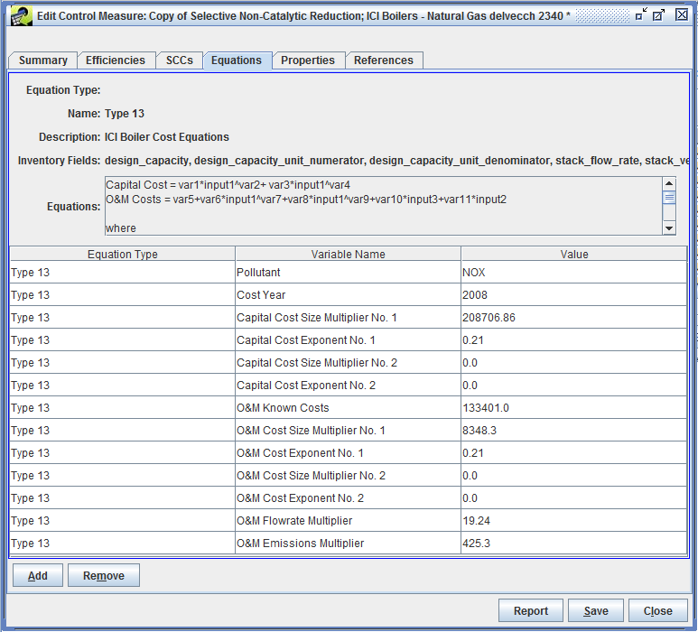
Step 4-13: Remove Control Measure Equation Data. To remove all of the equation information, click the Remove button. You will see a dialog that says “Are you sure you want to remove the equation information?”. To demonstrate how removing and resetting equation information works, click Yes to remove the equation information. All of the equation information will be removed from the Equations tab.
Step 4-14: Add Control Measure Equation Data. To add equation information to a measure, click the Add button on the Equations tab. You will see a Select Equation Type dialog. Click the pull-down menu to see the available types of equations and select the desired equation type. For this exercise, select Type 1 - EGU and click OK. You will see that there are eight variables for this equation type. Note that the variables differ somewhat from the variables for the Type 13 equation shown in Figure 3.23, and that the Type 1 equation is for NOx controls.
Details on the types of cost equations and their variables are given in the Documentation of Cost Equations in the EPA’s Control Strategy Tool (CoST).
For this exercise, click the Remove button again and click Yes to confirm removal of the equation information. Click the Add button on the Equations tab and select Type 13 - ICI Boiler Cost Equations. Next, fill in the values for the variables as they are shown in Figure 3.23 by double clicking on the field corresponding to each value and then entering the appropriate information.
Note: You can enter cost equations in terms of only one pollutant, even if the measure reduces emissions for multiple pollutants.
Click Save at the bottom of the Edit Control Measure window to save the changes you made to the control measure and to close the window. To see the revised name and abbreviation for the new measure, click the Refresh button at the upper right of the Control Measure Manager to load the updated data from the server.
Step 4-15: Edit Control Measure Properties. Go to the Properties tab of the Edit Control Measure Window (Figure 3.24). The buttons on the Properties tab of the Edit window are different from those on the View window. The available buttons are Add, Edit, and Remove. The property record allows for freeform property metadata/information to be associated with the measure. The property can be assigned a category grouping (e.g., Steam Factors), units (e.g., MW/hr), and a data type (e.g., numeric).
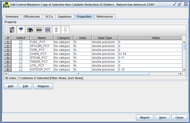
To edit a property record, scroll down to the COST_BASIS property, and check the corresponding checkbox in the Select column for the COST_BASIS property and then click Edit. The Edit Property Record window will appear (Figure 3.25). The data type is text, which means the property will contain textual information about the measure. Note also how the value field contains detailed information about the methodologies used for costing this control measure.
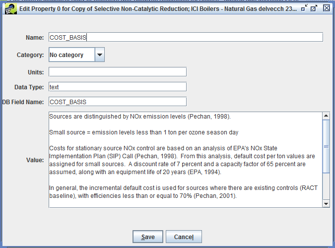
Edit the value for the property record as needed to reflect the new control measure. For this exercise, add some additional text to the Value, then click Save.
Step 4-16: Add a New Control Measure Property. To add a new property record, click Add in the Propertiestab. Fill in the appropriate values in the Add Property Record window that appears. For this exercise, set the Name to “POWER_LOSS”, select No category as the Category, MW/hr for the Units, numeric for the Data Type, POWER_LOSS for the DB Field Name, and 5 as the Value. Click Save once this information is entered and a new row will appear in the table in the Edit Control Measure window.
Step 4-17: Remove a New Control Measure Property. To remove one or more property records, click the corresponding checkboxes and then click Remove. For this exercise, click the checkbox in the Select column for POWER_LOSS and then click Remove and confirm with Yes to remove that record. The POWER_LOSS record will disappear from the table.
Step 4-18: Edit Control Measure References. Go to the References tab of the Edit Control Measure Window (Figure 3.26). The available edit buttons in this window are Add, Edit, and Remove.
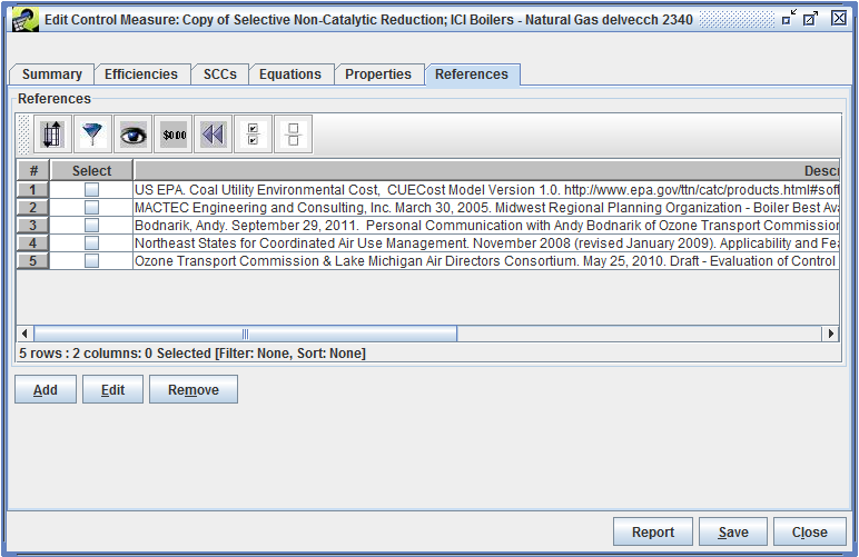
To edit an existing reference record, check the corresponding checkbox in the Select column and click Edit. For example, click the box next to the “MACTEC Engineering and Consulting…” reference entry and then click Edit. The Edit Reference Record window will appear (Figure 3.27).
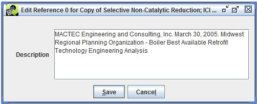
Edit the value for the reference record as needed to reflect information for the new control measure. For this example, add some additional text to the Description box, then click Save.
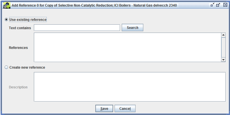
Step 4-19: Adding Control Measure References. To add a new reference for a control measure, click Add in the References tab, and the Add Reference Record window will appear (Figure 3.28). Either choose a reference that already exists in the database, or add a new reference.
To choose an existing reference, click on theUse existing reference option and then search for the reference by filling in the Text contains field, then click Search. When you have located the correct reference, select the item in the References box and click Save to add the reference to the control measure.
To create a new reference, click on the Create new reference option and then type the reference in the Description field, then click Save to add the reference to the control measure. For this exercise, click on Create new reference and then add “sample technical reference” to the Description field. Click Save and a new row will appear in the References table in the References tab of the Edit Control Measure window.
Step 4-20: Remove Control Measure References. To remove one or more reference records in the References tab, click the checkbox(es) next to the reference(s) to remove and then click Remove. For this exercise, click the checkbox in the Select column for the record for “sample technical reference” that you just added and click Remove and Yes to confirm to remove that record. The record will disappear from the references table.
Click Save at the bottom of the Edit Control Measure window to save the changes you made to the control measure and to close the window.
This section describes how to create new CoST control measures through the Control Measure Manager.
Step 5-1: Add a New Control Measure. To create a new control measure, click New on the Control Measure Manager to display the New Control Measure window as shown in Figure 3.18, except with none of the control measure information filled in.
Step 5-2: Adding a New Control Measure: Summary. Enter a unique name (e.g., New PM10-PRI Control Measure) in the Name field and a unique abbreviation (e.g., PNCM) in the Abbreviation field for the control measure. You must also set the Major Pollutant (e.g., PM10-PRI) and Class (e.g., Known) and the Date Reviewed for the measure before the measure can be saved into the CMDB. For more information on the fields in the Summary tab, see Viewing Data for an Existing Control Measure and Editing Control Measure Data above.
Step 5-3: Adding a New Control Measure: Efficiencies. Go to the Efficiencies tab of the New Control Measure window and add at least one efficiency record for the measure; otherwise it will have no effect on any emissions sources. The efficiencies tab for the new measure will look similar to Figure 3.19, except initially there will be no efficiency records. For more information on the data needed for efficiency records, see Viewing Data for an Existing Control Measure and Editing Control Measure Data. Add as many efficiency records as needed to describe the control efficiency and cost of the measure.
Step 5-4: Adding a New Control Measure: SCCs. Go to the SCCs tab of the New Control Measure window and add at least one SCC record for the measure; otherwise it will have no effect on any emissions sources. The SCC tab for the new measure will look similar to Figure 3.21, except initially there will be no SCC records. Note that the same control efficiency and cost information must apply to all sources with SCCs listed on this tab, otherwise the information must be stored in a separate measure for the other SCCs. For more information on the data needed for SCCs, see Viewing Data for an Existing Control Measure and Editing Control Measure Data.
Step 5-5: Adding a New Control Measure: Equations. To associate a cost equation with the new measure, go to the Equations tab and add an equation. The tab should look similar to the one shown in Figure 3.23. Cost equations are optional. If you do not have a cost equation, cost per ton information from one or more of the efficiency records will be used to estimate the cost of applying the measure.
Step 5-6: Adding a New Control Measure: Properties and References. To associate a property with the measure, go to the Properties tab and add a property. The tab should look similar to the one shown in Figure 3.24. Properties are optional.
To associate a reference with the measure, go to the References tab and add a reference. The tab should look similar to the one shown in Figure 3.26.
After all of the relevant information for the measure has been entered, click Save at the bottom of the New Control Measure window.
Step 5-7: View the New Control Measure. Set the Pollutant Filter in the Control Measure Manager to a pollutant specified for one of the new measure’s efficiency records (e.g. PM10-PRI), and you will see the new measure listed in the Control Measure Manager window. If you do not see it, try clicking the Refresh button to reload the measures from the server.
If the SCCs are known for a source, the Find button on the Control Measure Manager (e.g., see Figure 3.4) can be used to display which control measures are available for sources with those SCCs.
Step 6-1: Find Control Measures for SCCs. Before using the Find feature, set the Pollutant Filter (in the top left corner of the Control Measure Manager) to Select one, and click the Reset button on the toolbar, so that no pollutant or other filters will be applied prior to performing the next step. Click the Find button. You will see the Select SCCs window, similar to the one shown in Figure 3.22, except that all 11,900+ SCCs will be shown.
Use the Filter Rows button on the toolbar of the Select SCCs window to enter a filter that will help identify SCCs for which you would like to see available control measures. For this example, click Add Criteria twice and add the filters SCC starts with 103 and SCC starts with 305006, select Match using ANY criteria, and click OK. You should see 83 SCCs that meet this criterion.
Click the checkbox in the Select column for a few of the SCCs (e.g., select at least 10300101 and 30500606) and then click OK. If there are measures available for the selected SCC(s), they will be shown in the table. If you selected an SCC for which there are no measures available, none will be shown.
Click Find again and enter a filter on the Select SCCs window based on the SCC description instead of the SCC itself. For example, use the Filter Rows button on the Select SCCs window toolbar to enter the filter description contains Cement, then click on the checkbox in the Select column for a few of these SCCs (e.g., 30500606) and click OK. If there are measures in the database for the selected SCCs, they will be shown in the Control Measure Manager table. Note that there may be some SCCs for which there are no measures available in the database. In that case, no measures would be shown in the table after applying the SCC filter. For the measures that are returned, notice whether they all have the same value for Pollutant (e.g., measures for SCC 30500606 target NOx, PM10-PRI, and SO2).
The Pollutant pull-down menu near the bottom of the Control Measure Manager selects the pollutant for which the CPT, Control Efficiency (CE), Rule Effectiveness, and Rule Penetration data are shown in the Control Measure Manager. Note that to view these fields Show Details must be checked and you may need to scroll right or widen the window. Recall that each control measure can have efficiency records for multiple pollutants. By setting the Pollutant Filter at the top of the window, any measures that controls the selected pollutant will be shown in the table. The Pollutant pull-down menu displays the specific setting for the selected pollutant.
Step 7-1: Use the Pollutant Menu. To see the effect of the Pollutant pull-down menu, click the Reset button on the Control Measure Manager toolbar to remove any previously specified filters. Set the Pollutant Filter to PM25-PRI and make sure that Show Details? is checked. Set the Pollutant menu at the bottom of the window to MAJOR.
Examine the values in the Avg CPT, Min CPT, Max CPT, Avg CE, Min CE, and Max CE columns for some of the measures. Notice that for some of the measures, PM25-PRI is not the pollutant listed in the Pollutant column (e.g., sort on the Pollutant column by clicking on it once or twice to find other pollutants). These measures are shown in the manager because they all apply to PM25-PRI, even if PM25-PRI is not the major pollutant for the measure. In this case, the CPT and CE values are shown for the major pollutant specified for the measure, not necessarily for PM25-PRI.
Change the value of the Pollutant menu to something other than MAJOR (e.g., PM10-PRI). All entries in the Pollutant column are now set to the pollutant specified in the Pollutant menu, and the cost per ton (CPT) and control efficiency (CE) values are specific to the selected pollutant instead of being for the major pollutant specified for the measure. Note that CPT values may not be filled in for some measures. For PM measures, the cost information is typically associated with PM10-PRI, as opposed to PM25-PRI. Therefore, if the Pollutant menu is set to PM25-PRI, fewer CPT values will be shown than when Pollutant is set to PM10-PRI.
The Cost Year pull-down menu near the bottom of the Control Measure Manager controls the year for which the cost data are shown in the Manager. The default cost year is 2013. The cost data are converted between cost years using the Gross Domestic Product (GDP): Implicit Price Deflator (IPD), issued by the U.S. Department of Commerce, Bureau of Economic Analysis. Details of the computation used are given in the “Control Strategy Tool (CoST) Development Document.”
Step 8-1: Change the Cost Year. Change the cost year in the Cost Year menu from 2013 to an earlier year (e.g., 2010). Note how the CPT values decrease. If the cost year is changed to a later year, the CPT values increase.
Note that due to the method used to convert the costs between years, it is not possible to show costs for a future year (e.g., 2025); costs can be shown only for years prior to the current calendar year. The Cost Year cannot be set to the current calendar year because the economic data needed to make adjustments is not made available until after the end of each calendar year.
If an equation is specified for a measure, and there are no default CPT data available for that measure, the CPT will not be shown in the Control Measure Manager because it must be applied to an emissions source for the cost to be computed.
Control measure data can be exported from the Control Measure Manager to a set of CSV files. First identify a set of control measures for which to export data. Measures may be exported based on specifically selected control measures via the Control Measure Manager, or an entire set of measures associated with a certain sector may be exported.
Step 9-1: Export PM10-PRI Control Measures. To export measures that control PM10-PRI, set the Pollutant Filter on the Control Measure Manager to PM10-PRI. Next, use the Filter Rows button the toolbar to enter the following criterion: Name contains Fabric Filter. The Manager will display 44 measures.
Click the Select all button on the Control Measure Manager toolbar, and then click the Export button. The Exporting Control Measures window (Figure 3.29) will appear.
To export by selected measures, select the Export By Measure option. The list of measures displayed for export are the same measures that were chosen from the Control Measure Manager. Note it’s not necessary to click the “Select” checkboxes for these measures, all measures shown in the list will be exported regardless if they are checked or not. To export by inventory sector, select the Export By Sector option, then choose the various sectors for which to export control measures.
For this exercise, select Export By Measure to export the preselected measures from the Control Measure Manager. To specify the output folder (i.e., directory) into which the CSV files will be written, type the folder name into the Server Export Folder text field or use the Browse button to bring up a file and directory browser to select the output folder. To specify an export file name prefix for naming the new exported files, type the prefix string into the File Name Prefix text field.
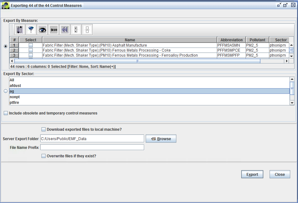
Type an export file prefix string (e.g., fabric_filter) into the File Name Prefix field of the Exporting Control Measures window. This string will be included at the beginning of the names of the exported CSV files to help identify the types of measures that are included in the files.
After setting the desired output folder and the file name prefix on the Exporting Control Measures window, click the Export button. The message at the top of the Export window will state that the export has started and to monitor the Status window to track the export request.
The Status, or Downloads, window is near the bottom of the EMF main window. It will show a message when the export starts and another when it is finished. Monitor the status on demand by clicking the Refresh button at the top of the Status/Downloads window.
Step 9-2: View the Exported Control Measures. After the export is finished, close the Exporting Control Measures window by clicking Close. Use your computer’s file browser to view the contents of the folder that you selected for the export. In the example shown above, the files created in the selected folder are: fabric_filter_summary.csv, fabric_filter_efficiencies.csv, fabric_filter_SCCs.csv, fabric_filter_equations.csv, fabric_filter_Props.csv, and fabric_filter_Refs.csv. These files may be opened with standard spreadsheet software. For a complete description of the fields in the files, see “Control Strategy Tool (CoST) Control Measures Database (CMDB) Documentation.”
Files in the exported format can also be imported into the CMDB. Control measures can only be imported to CoST/EMF by an Administrator.
Step 9-3: Import Control Measures. If logged in as Administrator, click the Import button on the Control Measure Manager to start importing measures. In the Import Control Measures window that appears (Figure 3.30), type or paste the name of the import Folder. You may also use the Browse button to browse to a folder containing the files to be imported and select the files directly from the browser. Alternatively, enter the folder name and then type in a pattern to specify the files, then click Apply Pattern. When using a pattern, an asterisk (*) will be expanded to the available file names.
After selecting the files to import, click the Import button. Information about the status of the import will be shown in the Status section of the window. To see updates to the status of the import, click the Refresh Import Status button. Once the imports are complete, click the Done button. If the measures already existed in the database, the new data will replace the existing data.
Note that as there will be no warning before the CMDB data are replaced, use the import feature with caution.
It is possible to purge existing measures from the CMDB by sector. This feature will remove all measures associated with the sectors chosen in the Purge Existing Measures By Sectors list. The user must also click the Purge checkbox to allow the measures to be purged. The measures will be purged when the Import button is clicked.
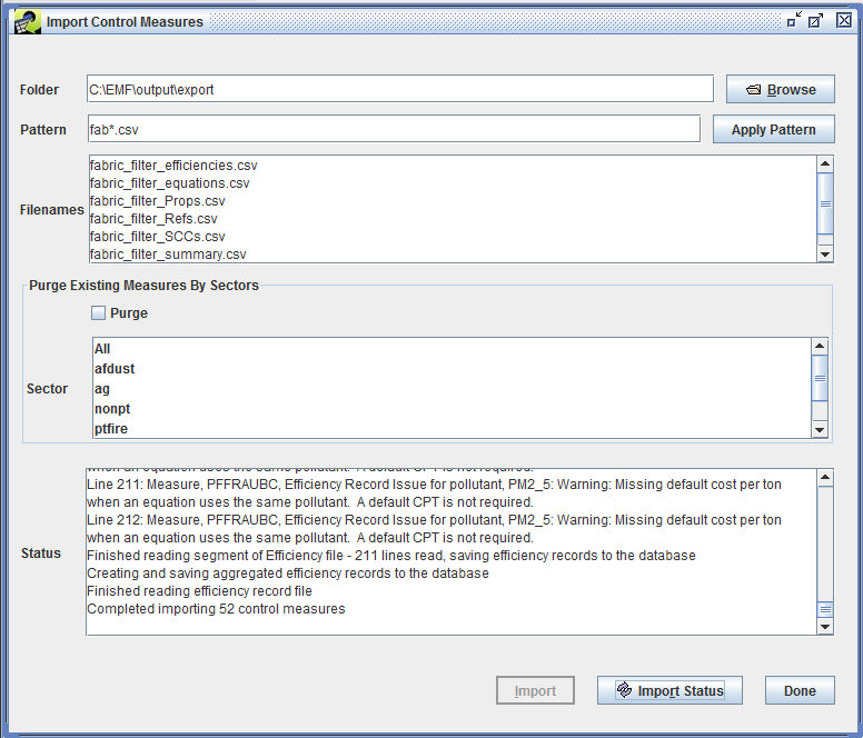
This chapter demonstrates the features of the Control Strategy Manager. The Control Strategy Manager allows control strategies to be created, edited, copied, and removed. A control strategy is a set of control measures applied to emissions inventory sources (in addition to any controls that are already in place) to accomplish an emissions reduction goal. Such goals are usually set to improve air quality and/or to reduce risks to human health. In this chapter, you will learn how to:
This chapter is presented as a series of steps so that it may be used as part of a training class or as a tutorial on how to use CoST. The numbered steps are the ones you are expected to perform, while other material is provided for documentation purposes.
CoST automates the key steps for preparing control strategies. The purpose of developing control strategies is to answer questions about which sources can be controlled and how much the application of those controls might reduce emissions and how much it might cost. For example, if the goal is to reduce NOx emissions for the Southeast U.S. in 2030 by 100,000 tons per year, CoST can help answer questions related to this goal, such as:
A future goal for CoST is to be able to answer this question: What is the optimum method for achieving simultaneously targeted reductions for multiple pollutants?
CoST can help answer the above questions when users set up and run one or more control strategies. A diagram of the basic steps for running a control strategy is shown in Figure 4.1. As illustrated in the figure, the inputs to a control strategy consist of:
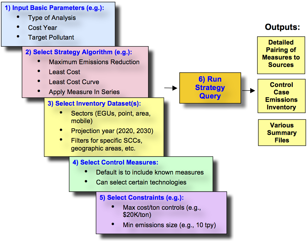
After a control strategy run is complete, several outputs are associated with the strategy. The main CoST output for each control strategy is a table called the “Strategy Detailed Result.” This table consists of emissions source-control measure pairings, each of which contains information about the cost and emissions reductions that would be achieved if the measure were to be applied to the source. If multiple inventories were processed by the strategy, then there will be one Strategy DetailedResult for each input inventory, unless the inventories were merged for a least cost run (as indicated in the ‘Multiple Inventories’ column Table 4.1). Also, there will be at least one Strategy Detailed Result for each of the least cost iterations performed as part of a Least Cost Curve run. In addition to the Strategy Detailed Result, two other outputs are produced for each strategy run: the Strategy County Summary (which includes uncontrolled and controlled emissions), and the Strategy Measure Summary (which summarizes how control measures were applied for each sector-county-SCC-Pollutant combination). These three outputs are referred to in Table 4.1 as the ‘Standard’ outputs.
The Strategy Detailed Result table itself can be summarized in many ways using predefined summary queries (e.g., by state, by county, by control technology). Users familiar with SQL can also define their own custom queries. The Strategy Detailed Result table can also be merged with the original input inventory, in an automated manner, to produce a controlled emissions inventory that reflects implementation of the strategy. The controlled emissions inventory includes information about the measures that have been applied to the controlled sources and can be directly input to the SMOKE modeling system to prepare air quality model-ready emissions data. Comments are placed at the top of the inventory file to indicate the strategy that produced it and the settings of the high-level parameters that were used to run the strategy.
Detailed information on the types of control strategy algorithms is provided in CoST Control Strategy Algorithms. Managing Control Strategies describes how to set up and manage control strategies. Inputs to Control Strategies details the inputs to control strategies, including adding inventories, control measures, and constraints to a strategy. Running a strategy and accessing its outputs are discussed in Running a Strategy and Accessing Its Outputs. Documentation for the various types of strategy outputs is given in Outputs of Control Strategies and information about summaries of strategy inputs and outputs is given in Summaries of Strategy Inputs and Outputs.
Once the inputs have been defined, the strategy can be run on the EMF server. The method by which the measures are associated with the strategies depends on the algorithm that has been selected for the strategy. At this time, four algorithms are available to determine how measures are assigned to sources:
Some of the key aspects of each of the strategy types are summarized in Table 4.1, and some additional information on each strategy type is provided in the following subsections.
| Strategy Type | Multiple Inventories | Typical Sectors | Measure Assignment | Outputs |
|---|---|---|---|---|
| Least Cost | Will be merged | Area, nonpoint | One per source | Standard, Least Cost Control Measure Worksheet |
| Least Cost Curve | Will be merged | Area, nonpoint | One per source | Standard, Least Cost Control Measure Worksheet, Least Cost Curve Summary |
| Maximum Emissions Reduction | Processed independently | Area, nonpoint | One per source, to achieve maximum reduction of target pollutant | Standard |
| Multi-Pollutant Maximum Emissions Reduction | Processed independently | Area, nonpoint | One per source target pollutant; based on specified target pollutant order; could be multiple per source | Standard |
The Maximum Emissions Reduction control strategy is the simplest of the strategy algorithms. It assigns to each source the single control measure that provides the maximum reduction to the target pollutant, regardless of cost. The strategy produces the three standard types of strategy outputs, including a Strategy Detailed Result for each input inventory.
The Least Cost control strategy type assigns measures to emissions sources to achieve a specified percent reduction or absolute reduction of a target pollutant for sources in a specified geographic region while incurring the minimum possible annualized cost. This algorithm is similar to the maximum emissions reduction control strategy in that only a single measure is applied to each source. For example, one measure might be selected for a source when trying to reduce the target pollutant by 20%. However, if you were trying to obtain a 40% reduction of the target pollutant, another more expensive measure that achieves a higher level of control might be selected for the same source to meet the targeted level of reduction. If multiple inventories are specified as inputs to a Least Cost control strategy, they are automatically merged into one EMF dataset as an ORL Merged dataset type. This allows the multiple inventory sectors to be considered simultaneously during a single Least Cost run. Note that the merged inventory dataset will be truncated and repopulated at the start of each strategy run, to ensure that the most up-to-date inventory data are included in the run.
The Least Cost control strategy automatically creates the same three standard output datasets, but it also creates an additional output dataset called the Least Cost Control Measure Worksheet. This output is a table of all possible emissions source-control measure pairings (for sources and measures that meet the respective filters specified for the strategy), each of which contains information about the cost and emissions reductions achieved if the measure was to be applied to the source. Examples of these tables are given in Outputs of Control Strategies. This dataset will be used to help generate a single Strategy Detailed Result (no matter how many input inventories were processed) once the optimization process has been performed to achieve the desired reduction. This dataset has the all of the same columns as the Strategy Detailed Result (see Table 4.9), in addition to the following columns:
marginal cost = annual cost (for specified cost year) / emissions reductions (tons)
Note that cost equations are used to compute the annual cost, when applicable and all required input data are available. For target pollutant source-control pair records, the annual cost will be the total of the annual costs for the target pollutant and any costs associated with co-pollutant reductions.
If multiple input inventories are used for the least cost control strategy run and the user requests to create controlled inventories, there will be one controlled inventory created for each of the input inventories.
The purpose of the Least Cost Curve control strategy type is to iteratively run Least Cost control strategies so that a cost curve of can be generated. In such cost curves, the cost per ton of emissions reductions increases as the level of desired emissions reductions increase. The input inventories are treated in the same way as the least cost run in that the data from the inventories will be put together into an ORL Merged inventory prior to performing any of the runs. The inventory filters and measure filters work in the same way as they do for the other strategy types, as do the constraints that apply to all strategy types. The main difference between the Least Cost and Least Cost Curve control strategy types is in the specification of constraints. Instead of specifying a single percent reduction or absolute emissions reduction, three new constraints are used to control the run:
Additional runs can be added to a least cost curve control strategy if you do not delete the previous results when you rerun the strategy. Suppose that you generate a coarse cost curve (default increment is 25%) and you find an area of interest that bears further examination. You can then go back and specify different start, end, and increment percent reductions to obtain more information (e.g., start=80%, end=90%, increment=2%) about that portion of the curve.
The types of outputs for a Least Cost Curve control strategy are the following:
The Multi-Pollutant Maximum Emissions Reduction control strategy assigns to each source the single measure for each target pollutant that provides the maximum reduction, regardless of cost. This process is performed for each target pollutant in an order specified by the user (e.g., NOx first, PM10-PRI second, VOC third, and SO2 last). If a measure would control a pollutant that was already controlled by a previous target pollutant analysis iteration, that measure will be excluded from consideration during the source-measure matching process. For example, if measure ABC controlled NOx (the first analyzed target pollutant) and VOC, and during the next pollutant iteration (for VOC) measure DEF also controls NOx and VOC, this measure will not be considered because VOC emissions were already controlled by applying the ABC measure.
The inventory filter and county filter work differently for this control strategy than they do for the other strategy types. The inventory filter and county filter can be specified separately for each target pollutant, whereas for the other strategy types they are defined at the strategy level.
The Multi-Pollutant Maximum Emissions Reduction control strategy produces the three standard types of strategy outputs, including a Strategy Detailed Result for each input inventory.
Occasionally, two or more control measures can be tied when ranked by an individual control strategy. For example, in a Maximum Emissions Reduction Control Strategy, the control measure that achieves the maximum emissions reduction will be selected. If two measure achieve the same reduction, the measure with the lower overall cost will be selected. If both measures have the same emissions reduction AND the same cost, the control measure whose abbreviation comes first in the alphabet will be used.
The control strategies currently available within CoST are shown in the Control Strategy Manager. The Control Strategy Manager allows you to see information about control strategies, to create new control strategies, and also to edit, remove, and copy control strategies.
Step 3-1: Open Control Strategy Manager. To open the Control Strategy Manager, choose Control Strategies from the Manage menu on the EMF main window (Figure 4.2) and the Control Strategy Manager will appear (Figure 4.3).
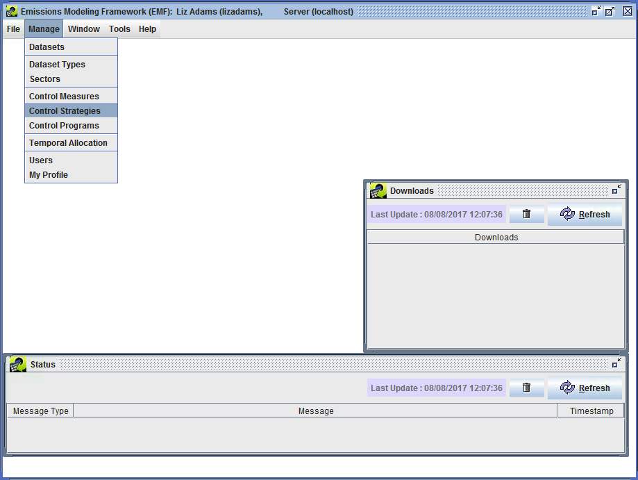
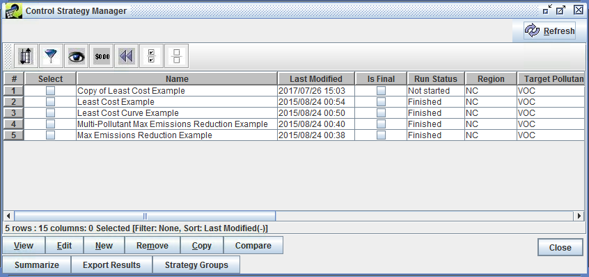
The Control Strategy Manager shows all of the control strategies currently available within the CoST/EMF system in a sortable, filterable window. The columns shown in the window are Select, Name, Last Modified, Is Final, Run Status, Region, Target Pollutant, Total Cost, Reduction (tons), Average Cost Per Ton, Project, Strategy Type, Cost Year, Inventory Year, and Creator. Descriptions of some of the columns are given in Table 4.2. The remaining fields are described in detail in Inputs to Control Strategies.
| Column | Description |
|---|---|
| Name | Shows the name of the control strategy. |
| Last Modified | Shows the date and time on which the strategy was last changed. |
| Run Status | Gives information about the strategy run. Possible options are: Not started - the strategy run has never been started; Waiting - a run has been requested, but it is waiting because other strategies are running; Running - the strategy is currently running; Finished - the strategy run completed successfully; Failed - the strategy run started, but failed due to a problem. |
| Inv Year | Shows the year of the emissions inventory that the strategy will process. |
By default, the strategies are shown using a descending sort on the last modified date and time, so that the most recently modified strategies appear at the top of the list.
Step 3-2: Sort Control Strategies. To sort the control strategies on the total cost of the strategy, click on the heading of the Total Cost column and the rows will re-sort so that the most expensive strategies will be shown at the top. Click on the Total Cost column header again to reverse the sort.
Step 3-3: Filter Control Strategies. To see only strategies that were run with a specific target pollutant, click the Filter button on the Control Strategy Manager toolbar. When the Filter Rows window appears enter a criterion for the filter by clicking Add Criteria. Click in the cell under Column Name and choose Target Pollutant. Change the operation by clicking in the cell under Operation. For this example select contains as the desired Operation. Enter the pollutant of interest in the Value cell. Enter PM25-PRI in the Value cell for this example.
Note that the filter values are case-sensitive (e.g., “NOx” will not match a filter value of “NOX”). After applying the filter criterion above, the Filter Rows window will look like Figure 4.4.
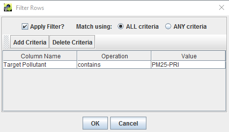
Click OK and the Control Strategy Manager will show only strategies that targeted PM25-PRI.
After reviewing the information available on the Control Strategy Manager for PM25-PRI measures, click the Reset button to remove the filter and sort criteria.
For more information on performing sorting, filtering, formatting, and other operations on the table that shows the control strategies used for the Control Strategy Manager, refer to the Introduction to the Control Measure Manager.
Existing strategies can be copied to create new control strategies, regardless of whether they have been run. If you copy a strategy and then edit the newly created strategy, you will not be changing any settings for the original strategy, so this is a safe way to start working with your own strategies. When a strategy is copied, it retains all of the settings from the original strategy except for the information on the Outputs tab, and the output summary information that is shown on the Summary tab.
Step 3-4: Copy Control Strategies. Click the Select checkbox next to one of the strategies (e.g., “Least Cost Example) and then click Copy. A new strategy will be added to the Control Strategy Manager with the name”Copy of original strategy name."
Note that multiple strategies can be copied at once by selecting as many strategies as needed before clicking Copy.
A control strategy creator and an EMF Administrator can remove control strategies from CoST. Strategies should be removed with caution, because there is no ‘undo’ for this operation.
Step 3-5: Remove Control Strategies. Click the Select checkbox next to one of the strategies and then click Remove. As an example, select the strategy you just copied in the previous subsection. When prompted to confirm removal of the control strategy, a pop-up menu will appear in Figure 4.5 where the user can select whether to remove output datasets associated with the strategy that they would like to remove. The first check box is to remove the following output data: Strategy results, messages, and summaries assocated with the control strategy that is being deleted. The second check box is to remove the Controlled inventories associated with the control strategy that is being deleted. Check both check boxes, so that all datasets created by the control strategy are cleaned up when the strategy is deleted. The selected strategy and output datasets will be removed from the table of strategies in the Control Strategy Manager.
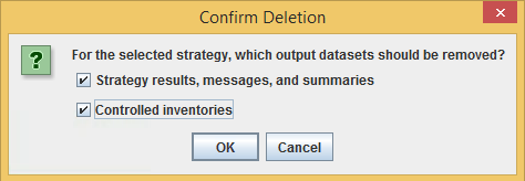
Note that if you select more than one control strategy before clicking Remove, all of the selected strategies will be removed.
Step 3-6: Create New Control Strategies. To create a new control strategy, click the New button in the Control Strategy Manager. The Create New Control Strategy window will appear with a text box to name the new strategy. Enter a name that is different from any of the existing control strategies (e.g., Least Cost 2017 NOx Example) and then click OK.
An Edit Control Strategy window for your newly created strategy will appear in Figure 4.6. The window has five tabs: Summary, Inventories, Measures, Constraints, and Outputs. This window and how to fill in the information on these tabs is discussed in more detail in Inputs to Control Strategies.
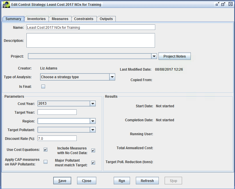
For this example, edit the following fields in the Edit Control Strategy window:
Target Year to 2017Type of Analysis to Least CostTarget Pollutant to NOXClick Save to save the new strategy and click Close to close the Edit Control Strategy window.
If the new strategy does not appear in the Control Strategy Manager, first click the Reset button on the toolbar to remove any filters that have been applied to the strategies. If the strategy still does not appear, click Refresh at the top right of the Control Strategy Manager to obtain new data from the server.
Step 3-7: Edit Control Strategies. Click the Select checkbox next to the new strategy (i.e., the strategy created in Step 3-6) and then click Edit. If you have permission to edit the strategy (i.e., you are its creator or an Administrator), the Edit Control Strategy window will appear with the Summary tab visible (Figure 4.7). Note that if you had selected multiple control strategies before clicking Edit, they each would have opened in their own window. The tabs on the Edit Control Strategy window are listed in Table 4.3. The contents of these tabs are described in detail in Inputs to Control Strategies.
| Tab | Description |
|---|---|
| Summary | Shows you high-level information about the strategy, such as its Name and the Target Pollutant. |
| Inventories | From which you can specify the emissions inventories to use as input to the strategy and filters for those inventories. |
| Measures | Allows you to specify the classes of measures to include in the strategy, or select specific measures to include. |
| Constraints | Allows you to specify constraints for the strategy, such as a maximum cost per ton. |
| Outputs | Shows the results from the strategy after it has been run. |
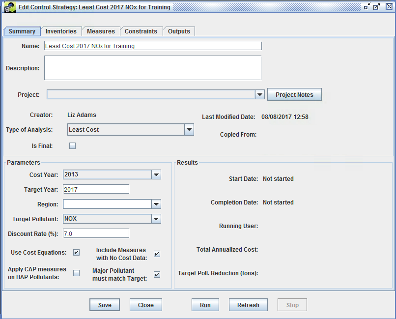
Control strategies are defined by a series of fields that must be set prior to running the strategy. These fields are described in this section.
Along with the name and description of the strategy, the Control Strategy Summary tab defines the type of analysis to use for the strategy, spatial-temporal parameters, the target pollutant, and the interest rate. To set the fields for the strategy on the Summary tab (see Figure 4.7), follow the steps below. Note that the fields on the Summary tab missing from this list are automatically set by CoST, and are discussed in Fields Automatically Set by CoST. Fields that are contained within boxes with either white backgrounds or that are pull-down menus are editable; fields that are not contained within boxes are set by the software and cannot be changed by the user.
Step 4-1: Set the Control Strategy Name and Description. If one has not already been specified, enter a unique and descriptive Name for the control strategy. For this example set Name to Least Cost 2017 NOx Example. Enter a Description of the purpose for the control strategy, and any other information relevant and useful to describe the strategy.
Optionally, use the Project pull-down menu to select a project for which this strategy run was performed (e.g., Ozone NAAQS Final 2008). Projects are set in the EMF and are used as a means of grouping related strategies that were performed in support of a common goal.
Step 4-2: Set Strategy Type. Use the Type of Analysis pull-down menu to set the type of algorithm used to match the control measures with sources (e.g., Maximum Emissions Reduction, Least Cost). For this example, select Least Cost as the analysis type.
Optionally specify whether the strategy Is Final to finalize and archive the strategy. Once marked as final, a strategy may not be rerun. For this exercise, do not check the Is Final checkbox.
Step 4-3: Set the Cost Year. Use the Cost Year pull-down menu to set the year to use for estimating the costs of a strategy. For this exercise, set Cost Year to 2013. All cost data specified for the control measures will be converted to this year using the Gross Domestic Product (GDP): Implicit Price Deflator (IPD), issued by the U.S. Department of Commerce, Bureau of Economic Analysis. Details of the computation used are given in the Control Strategy Tool (CoST) Development Document. The Cost Year cannot be set to the current year because the economic data necessary is not made available until after the end of each calendar year.
Step 4-4: Set the Target Year. The target year should correspond to the input inventory or inventories (e.g., 2020, 2030). For control measure efficiency records to be considered for a strategy, the specified effective date for the record must be equal to or earlier than the target year. Note that any control measure efficiency records that come into effect after the target year will not be considered for use in the strategy. For this example set Target Year to 2017.
Optionally set the name of the geographic Region to which the strategy is to be applied. This setting is informational only and does not impact the strategy results. Region is different from the concept of “locale” used in the control measure efficiency records to indicate the state or county code to which the record applies. For this example, set Region to NC.
Step 4-5: Set the Target Pollutant. The target pollutant is the pollutant of primary interest for emissions reductions from the control strategy. The Least Cost and Maximum Emissions Reduction algorithms will apply reductions to the target pollutant. For the Multi-Pollutant Maximum Emissions Reduction strategy, one or more pollutants must be selected from the Target Pollutant pull-down menu.
Note that reductions of pollutants other than the selected target pollutant (e.g., PM10-PRI, PM2.5-PRI, elemental carbon [EC], organic carbon [OC]) will be included in strategy results if those pollutants both appear in the inventories input to the strategy and they are affected by measures applied as part of the strategy. These pollutants are sometimes referred to as “co-impact pollutants”, because the impact on the emissions could be either a reduction (i.e., a benefit) or an increase (i.e., a disbenefit).
If Multi-Pollutant Maximum Emissions Reduction is selected from the Type of Analysis pull-down menu, set the Target Pollutant using the Set button next to this field to select from a list of pollutants to use for the strategy. Select the pollutants to include in the strategy from the pollutant list using Control-Click.
For this Least Cost example, use the pull-down menu to set Target Pollutant to VOC.
Step 4-6: Set the Interest Rate. The Interest Rate is used in the calculation of the annualized capital cost for control measures when appropriate data are available. For this example, set the Interest Rate to 7.0. Note that the interest rate typically does not affect strategies for area or mobile sources.
Step 4-7: Use Cost Equations. When the Use Cost Equations checkbox is checked, cost equations will be included in the strategy run; otherwise only cost per ton-related (CPT) cost estimates will be used. For this exercise, leave Use Cost Equations checked to use the Least Cost equations selected as the Type of Analysis in Step 2-9.
Step 4-8: Apply CAP measures on HAP Pollutants. When the Apply CAP measures on HAP Pollutants checkbox is checked, a CAP-to-HAP pollutant mapping is used to apply CAP reductions to the corresponding HAP pollutants at the same emission reduction percentage. For this exercise, leave Apply CAP measures on HAP Pollutants unchecked so that HAP pollutant controls will not be used.
Step 4-9: Include Measures with No Cost Data. When the Include Measures with No Cost Data checkbox is checked, measures with control efficiencies but without cost data are included in the strategy run; otherwise they are not included. These are typically measures with no cost data specified or measures that use a cost equation to compute cost, but for which there is not enough data for the source in the inventory to fill in the equations variables. For this exercise, leave Include Measures with No Cost Data checked.
Step 4-10: Specify whether Major Pollutant must match Target. When the checkbox is checked, then the major pollutant must be the same as the target. For this exercise, leave Major Pollutant must match Target checked.
Some fields of a control strategy that appear on the Summary tab are set automatically by the CoST software and are not specified by the user. Note that some of these summarize the results of the strategy analysis, so information for them is not available until after the strategy has been run. The automatically set fields are described in Table 4.4.
| Field | Description |
|---|---|
| Creator | The name of the person who created the strategy. |
| Last Modified Date | The date and time when the strategy was last modified. |
| Copied From | The name of the strategy that this strategy was copied from, if any. |
| Start Date | The date and time on which the strategy run was most recently started, or “Not started” if the strategy has never been run. |
| Completion Date | The date and time on which the strategy run was most recently completed. If the run has not completed, this field shows the run status of either “Not started”, “Running”, “Waiting”, “Completed”, or “Failed”. |
| Running User | The name of the user who most recently ran the strategy. |
| Total Annualized Cost | The total annualized cost of applying the strategy. |
| Target Poll. Reduction (tons) | The absolute emissions reduction achieved for the target pollutant, in tons. |
This section describes how to set the inventory inputs for a Control Strategy on the Edit Control Strategy window Inventories tab (Figure 4.8). Click on the Inventories tab. The Inventories to Process table near the top of the tab lists the emissions inventories for which the control strategy will be run. A control strategy can have one or more emissions inventories as input. Before inventories can be selected for use in the strategy, they must already have been imported into the EMF using either the Import item on the File menu of the EMF Main Window or through the Dataset Manager. The CoST application comes preloaded with several example inventories for training purposes.
CoST/EMF supports both one-record-per-line (ORL) and flat file (FF10) inventory formats. Point source inventories have information about emissions sources with specific locations, which are specified using latitude and longitude. Nonpoint, nonroad, and onroad inventories contain data aggregated to the county level. Note that IDA inventories are not supported by CoST and need to be converted to ORL or FF10 prior to use with CoST. The EMF database stores the data for the emissions inventories along with metadata about the inventories in its PostgreSQL (http://www.postgresql.org) database.
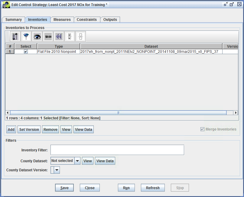
Step 4-11: Add an Inventory to Control Strategy. To add one or more inventories to the Inventories to Process table for the control strategy, click the Add button on the Inventories tab. From the Select Datasets window that appears, use the Choose a dataset type pull-down menu to select the type of inventory to add (e.g., Flat File 2010 Nonpoint). The file browser will display the inventories of the specified type (Figure 4.9). If there are many inventories in the list, narrow down the list (e.g., to find inventories for 2017) by entering a search string in the Dataset name contains field and pressing the Enter key on your keyboard.
To select an inventory to use for the strategy from the Select Datasets window, click on the name of the inventory in the table. For this exercise, after choosing Flat File 2010 Nonpoint from the Choose a dataset type pull-down menu, select 2017eh_from_nonpoint_2011NEIv2_NONPOINT_20141108_09mar2015_v0_FIPS_37 and then click OK. The inventory file will then be displayed in the Inventories to Process window of the Inventories tab.
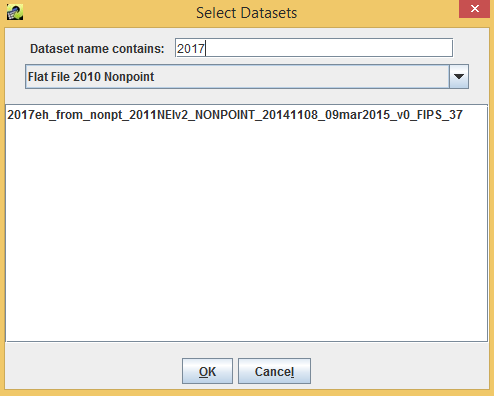
Step 4-12: Add a Second Inventory to Control Strategy. Click the Add button to add a second inventory to the control strategy. Select Flat File 2010 Point from the Choose a dataset type pull-down menu and add 2017eh_from_ptnonipm_2011NEIv2_POINT_20140913_revised_20150115_10mar2015_v0_FIPS_37.
Note: To select multiple inventories, hold down the control key while clicking the additional inventories.
Step 4-13: Remove an Inventory from a Control Strategy. To remove inventories from a control strategy, click the Select checkbox next to the inventory to remove and click the Remove button below the Inventories to Process table (Figure 4.8). Click Yes to confirm deletion of the selected inventories. There is no need to remove either of the inventories for this example strategy.
Step 4-14: Set Dataset Versions. Note that multiple versions of the inventories may be available within the EMF. The EMF supports dataset versioning to facilitate reproducibility of historical runs. To specify which version of an inventory to use, check the Select checkbox next to a single inventory file in the Inventories to Process table and then click the Set Version button. A window will appear with a pull-down menu that lists the versions available for the selected inventory. Choose the desired version from the menu and then click the OK button to set the version to use for the strategy. You will then see the version number in the Version column of the Inventories to Process table. Note that the initial version of a dataset is always version 0. There is no need to change the inventory versions for the example exercises.
Step 4-15: View Dataset Properties. To see the properties (i.e., metadata) for an inventory dataset, click the checkbox in the Select column of the Inventories to Process table and then click View. The Dataset Properties View window will appear (Figure 4.10). The Dataset Properties View window provides information about the selected inventory dataset and has multiple tabs as described in Table 4.5.
| Tab | Description |
|---|---|
| Summary | Shows high-level properties of the dataset |
| Data | Provides access to the actual inventory data so that you can view the data that will be used in the control strategy |
| Keywords | Shows additional types of metadata not found on the Summary tab |
| Notes | Shows comments that users have made about the dataset and questions they may have |
| Revisions | Shows the revisions that have been made to the dataset |
| History | Shows how the dataset has been used in the past |
| Sources | Shows where the data came from and where it is stored in the database, if applicable |
| QA | Shows QA summaries that have been made of the dataset (e.g., state summaries, county summaries) |
In addition to the different tabs, there are buttons at the bottom of the Data Properties window. The Edit Properties button displays the Dataset Properties Editor for changing (as opposed to viewing) the properties of the Dataset. The Edit Data button displays the Dataset Versions Editor for editing the actual data of the dataset by adding new versions. The Refresh button updates the data on the Dataset Properties View window with the latest information available from the server. The Export button exports the dataset data to a file. The Close button closes the Dataset Properties View window.
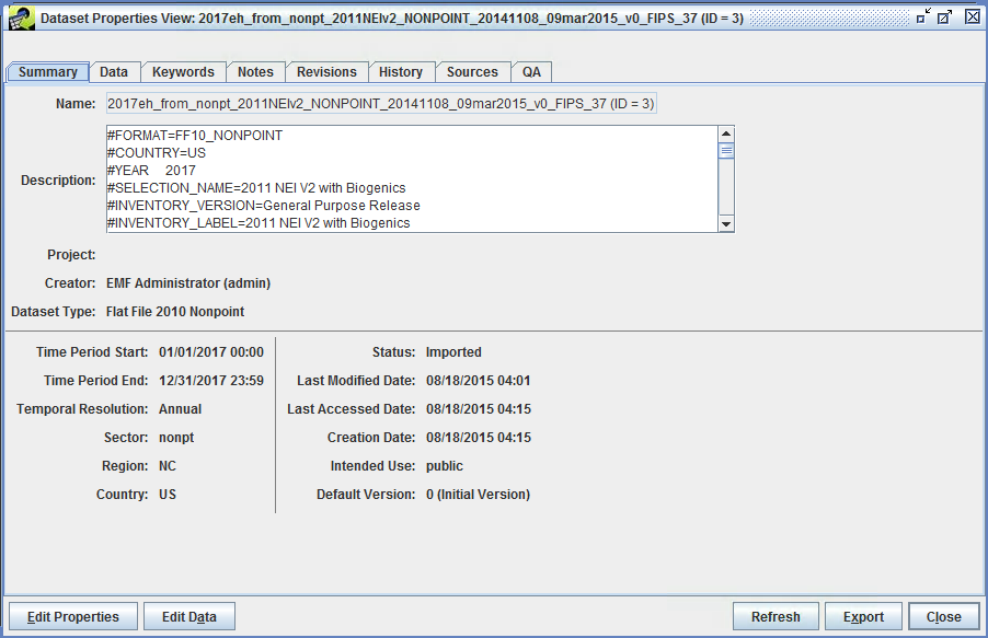
Close the Dataset Properties View window by clicking Close.
Step 4-16: View Inventory Data. To view the inventory data itself (as opposed to just the metadata), check the Select checkbox next to an inventory file in the Inventories to Process table in the Inventories tab of the Edit Control Strategy window and click the View Data button. A Data Viewer window will appear that shows the actual data for the selected inventory (Figure 4.11). The data shown here are different from the metadata in the Dataset Properties View window. Note that the View Data button is a shortcut. The Data Viewer can also be brought up from the Data tab of the Dataset Properties Viewer.
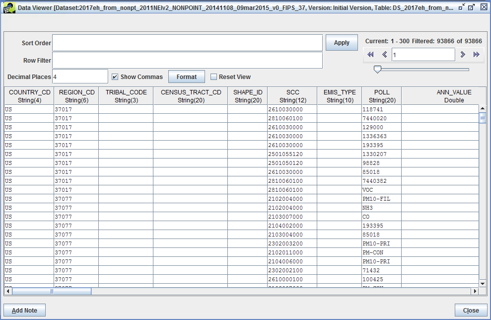
Inventories can contain a lot of data, so only the first 300 rows of an inventory are transferred from the server to the Data Viewer by default. The fields in the upper right corner of the window in the area labeled “Current” provide information about how many rows the inventory has, and which rows are currently visible. The Data Viewer works similarly to a web search engine that shows the results in pages, and the pagination arrows near the upper right corner of the window facilitate moving between pages of data. Use the pagination arrows in the upper right corner of the window to see how they work. Go to first record, go to previous page, give a specific record, go to next page, and go to last record.
The data sorting can be controlled by entering a comma-separated list of columns in the Sort Order field and then clicking Apply. Note that a descending sort order can be specified by following the column name with “desc” (e.g., ANN_VALUE desc, REGION_CD will sort by decreasing annual emissions and then by county).
If you enter a Row Filter, and then click Apply, the Data Viewer will find rows that meet the specified criteria. Examples of the syntax for row filters are given in Table 4.6. See Chapter 6 for additional row filter examples.
| Filter Purpose | SQL Where Clause |
|---|---|
| Filter on a particular set of SCCs | SCC LIKE '246%' OR SCC LIKE '261%' |
| Filter on a particular set of pollutants | POLL IN ('PM10-PRI','PM25-PRI')or POLL = 'PM10-PRI' OR POLL = 'PM25-PRI' |
| Filter sources only in NC (REGION_CD starts with 37); note that REGION_CD column format is State + County FIPS code (e.g., 37017) |
SUBSTRING(REGION_CD,1,2) IN ('37') |
| Filter sources only in NC (37) with county FIPS codes that start with 1 | REGION_CD LIKE '371%' |
| Filter sources only in NC (37) and include only NOx and VOC pollutants | SUBSTRING(REGION_CD,1,2) = '37' AND POLL IN ('NOX', 'VOC')or REGION_CD LIKE '37%' AND (POLL = 'NOX' OR POLL = 'VOC') |
Click Close to close the Data Viewer window.
The next few paragraphs provide information on how the options at the lower portion of the Inventories tab work.
Some control strategy algorithms (e.g., Maximum Emissions Reduction) are designed to process the inventories iteratively and produce results for each inventory. However, the “Least Cost” and “Least Cost Curve” strategy types can merge the input inventories from multiple sectors together prior to processing them, thereby facilitating cross-sector analyses. The Merge Inventories checkbox in the lower right corner of the Inventories to Process section of the Inventories tab controls whether multiple inventories will be merged together prior to applying the strategy algorithm, such as for Least Cost or Least Cost Curve runs. Otherwise, each inventory will be processed independently to create separate, independent results.
The fields in the Filters section of the Inventories tab of control whether the entire inventory is processed in the strategy or just a portion of it. The Inventory Filter field sets a general filter that can be entered using the same syntax as a Structured Query Language (SQL) “where clause”. Any of the columns in the inventory can be used in the expression. Examples include: SCC LIKE '212%' to limit the analysis to apply only to inventory records for which the SCC code starts with 212, and REGION_CD LIKE '06%' OR REGION_CD LIKE '07%' to limit the strategy analysis to apply only to inventory records with numeric state-county codes starting with 06 or 07. Additional examples of filters are shown in Table 4.6.
Note: for the Multi-Pollutant Maximum Emission Reduction control strategy type the Inventory Filter has been moved from the Inventories tab to the Constraints tab. (you are currently viewing the Least Cost Curve Strategy at this point in the exercise, so the Inventory Filter is on the Inventories tab) For the Multi-Pollutant Maximum Emissions Reduction control strategy it is possible to specify the Inventory Filter differently for each target pollutant instead of at the strategy level. Note that within the inventory filter, either upper or lower case may be used to refer to the column names and for the SQL keywords; the specified values within single quotes, however, are case sensitive (e.g., 'NOx' is different from 'NOX'). Adding an inventory filter will not have an effect on the strategy until the strategy is run.
If an inventory filter includes only specific pollutants, then pollutants not specified by the filter will not be considered for the computation of co-impacts from a strategy. In addition, pollutants like EC and OC that are not traditionally included in input inventories will not be included in the results unless the inventory has been preprocessed to include EC and OC.
The County Dataset filter allows another way to filter the inventory. This field sets an EMF dataset with a list of counties to which control measures will apply during the strategy run. Control measures will be applied only to counties that are included in this list. The County Dataset pull-down menu will show the names of the available CSV datasets in the EMF that have the dataset type ‘List of Counties (CSV)’. Note that CSV files from which these county datasets are created must have at least two columns of data. Also, the first row of the file must be the column names, and one of the columns must have a name that starts with “FIPS”. CoST will assume that this column has the list of FIPS codes that should be controlled. Make sure that leading zeros are present for FIPS codes less than 10000. Note that for the Multi-Pollutant Maximum Emissions Reduction control strategy type the County Dataset filter has been moved from the Inventories tab to the Constraints tab. For the Multi-Pollutant Maximum Emissions Reduction control strategy it’s possible to specify different County Dataset filters for each target pollutant instead of at the strategy level.
Note that only the records of the input inventories that pass both the inventory and county filters will be considered for control measure application.
Step 4-17: Set Inventory Filters. For this exercise, set the following on the Inventories tab: Inventory Filter: REGION_CD IN ('37077', '37017', '37095'). Note that specifying a list of counties using the Inventory Filter is an alternative to specifying a county dataset that has a list of counties to consider controlling in the strategy (as shown in the next bullet). To control only a few counties, it is straightforward to use the Inventory Filter; to control more than a few counties, the county dataset method is recommended. In addition, many types of Inventory Filters can be specified using other fields of the inventory depending on the specifications of the control strategy (e.g., SCC LIKE '231%', or ANN_VALUE > 5).
Step 4-18: View a County Dataset. Examine the available county datasets by pulling down the County Dataset menu and selecting one of the datasets. After selecting a county dataset, examine the dataset properties by clicking View. Display the actual county dataset data by clicking View Data. Select a version of the dataset using the County Dataset Version field, which shows the available versions of the selected dataset. This selection is required because the EMF can store multiple versions of each dataset.
For this example, set the County Dataset pull-down menu to Not selected before proceeding.
The Measures tab appears on the Edit Control Strategy window for all types of strategies. The Measures tab sets the control measures to use in a strategy run. There are two mutually exclusive ways to select control measures for inclusion in the control strategy run. The default is to include measures according to their class (see the top half of Figure 4.12). Currently available classes are Known (i.e., already in use), Emerging (i.e., realistic, but in an experimental phase), Hypothetical (i.e., the specified data are hypothetical), and Temporary (controls that are used during the analysis only if the user was the creator of the control measure, therefore other users’ temporary measures won’t be considered during an analysis). By default, only Known measures will be included in the strategy run. The second way to specify measures for inclusion in a strategy run is to select a list of specific measures to consider using for the run. The use of these two methods is described in this section. To select additional classes of measures other than the default ‘Known’, hold down the Ctrl key while clicking the desired classes of measures. To start over with selecting classes, just click on a single class of measure without holding down the Ctrl key. Note that only the measures with the classes selected by the user will be included in the strategy run.
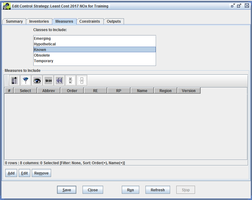
Step 4-19: Select Control Measures by Class. Click on one of the classes in the Classes to Include table and click Save to include all measures of a given class in a control strategy. To select multiple classes of measures, hold down the Ctrl key while clicking the desired classes of measures. To start over with selecting classes, just click on a single class of measure without holding down the Ctrl key. Note that only the measures with the classes selected by the user will be included in the strategy run.
Step 4-20: Select Specific Control Measures. To select specific measures for inclusion in the strategy, click the Add button under the Measures to Include table to show the Select Control Measures window (Figure 4.13). In this window, set a filter to find all measures with the same control technology. Use the checkboxes in the Select column to select the measures to include in a control strategy. To select all of the measures shown in the Select Control Measures window, click the Select All button in the toolbar. Uncheck measures to exclude from a strategy. For this example, use the Filter to select all sources matching the following criteria: Abbrev contains SNCR.
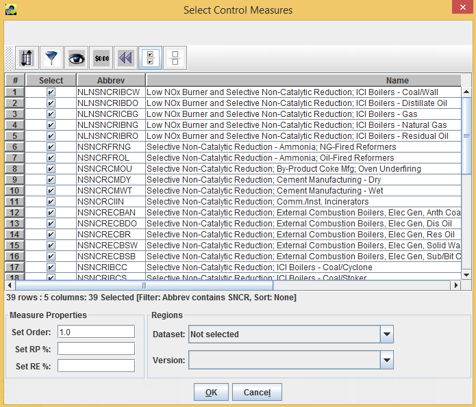
Set Order: Controls the order in which the current group of measures is applied as compared to other groups of measures selected for the control strategy. This option is not used by any current control strategies.Set RE%: Overrides the values of Rule Effectiveness specified in the measure efficiency records.Set RP%: Overrides the values of Rule Penetration specified in the measure efficiency records. These two settings are useful for assessing the level of emissions reductions achieved assuming different levels of effectiveness and penetration for the measures. For example, setting the rule penetration to 75% assumes that 75% of the sources are applying the measure and would therefore result in 75% of the emissions reductions it would achieve if it was 100%.Regions: Sets a county dataset from the Dataset pull-down menu and a version of that dataset from the Version menu. By setting a Region the selected measures will only be applied to counties listed in the selected county dataset.After selecting some the specific measures and overrides using the Select Control Measures window, click OK to add the measures to the control strategy. The selected measures will appear on the Measures tab. The tab will now look similar to that shown in Figure 4.14. Note that only the table of specific measures and their properties is shown, and the Classes to Include list is no longer shown. If desired, you may repeat the process of selecting specific measures to add new sets of measures to the list of measures to be used for the strategy. Each new group of measures selected can have different settings for the order, RE, RP, and Region.
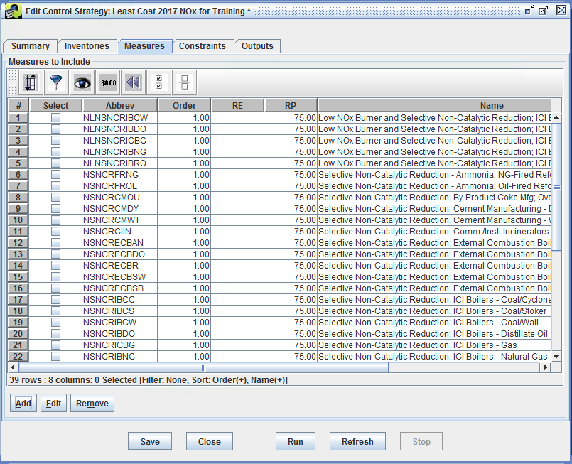
Step 4-21: Editing Control Measures List. Specific measures included in a control strategy can be changed by selecting the measure(s) to edit using the checkboxes in the Select column of the Measures to Include table in the Measures tab of the Edit Control Strategy window. Select the measures to change and click the Edit button. An Editing Measures window will appear that supports changes to the measure properties as they apply to the control strategy. Click OK to accept the edits or Cancel to reject the edits.
Step 4-22: Removing Control Measures from a Strategy. To remove specific measures from the list of measures to be included in a strategy run, check the corresponding Select checkboxes and then click Remove. Click Yes to confirm the removal of the selected measures from the control strategy.
For this example, remove all of the individually selected measures by clicking the Select All button on the Measures tab toolbar and then clicking Remove and Yes when prompted. Make sure that Emerging and Known are both selected in the Classes to Include list. The Measures tab will again look like Figure 4.12.
The Constraints tab (Figure 4.15) of the Edit Control Strategy window can be used to specify constraints for a control strategy to limit how control measures are assigned during the strategy run. For example, a strategy could be set up to not use any measures that cost more than $5,000 per ton (in 2013 dollars) for the target pollutant. Alternatively, a strategy could be defined to only use measures that reduce at least 1 ton of the target pollutant for the source. CoST evaluates the constraints while the source is being matched with the control measures. For example, the emissions reductions achieved by applying a measure to a source are not known until the measure and its control efficiency have been selected. Thus, constraint calculations are dependent on both the inventory source and the measure being considered for application to the source. Note that the term “source” here refers to a single row of the emissions inventory, which for point sources is uniquely determined by FIPS, plant, point, stack, segment, and SCC, and for nonpoint sources is uniquely determined by FIPS and SCC. Sources should not be confused with “plants”, each of which can contain many sources.
Table 4.7 defines the constraints that are applicable to all strategy types. If the constraint values are not satisfied for a particular control measure and source combination, the measure under consideration will not be applied to the source, and CoST will look for another measure that satisfies all of the constraints.
| Constraint Name | Constraint Description |
|---|---|
| Minimum Emissions Reduction (tons) | If specified, requires each control measure to reduce the target pollutant by at least the specified minimum tonnage for a particular source (down to the plant+point+stack+segment level of specification); if the minimum tonnage reduction is not attainable, the measure will not be applied. |
| Minimum Control Efficiency (%) | If specified, requires each control measure used in the strategy to have a control efficiency greater than or equal to the specified control efficiency for a particular source and target pollutant. |
| Maximum 2013 Cost per Ton ($/ton) | If specified, each control measure must have an annualized cost per ton less than or equal to the specified maximum annualized cost per ton for the target pollutant for each source. This cost is based on 2013 dollars. |
| Maximum 2013 Annualized Cost ($/yr) | If specified, each control measure must have an annualized cost less than or equal to the specified annualized cost for each source and target pollutant. This cost is based on 2013 dollars. |
| Minimum Percent Reduction Difference for Replacement Control (%) | If specified, each control measure must have a percent reduction in emissions with the new measure that is greater than or equal to the specified difference for the old control measure to be “replaced by” the new control measure. Incremental controls that add an additional device onto a currently controlled source are not yet supported by CoST. In the event that a combination of two control devices is listed as a control measure (e.g., LNB+FGR) and the combined control efficiency provides an ample increase in the control efficiency over the original efficiency, that combination of the devices can still serve as a replacement control if the source already has a measure applied (e.g., LNB). In the future, instead of requiring an increase in the percent reduction, it may be more useful to specify a minimum additional percent reduction in remaining emissions (e.g., such as one might see when going from a 99% control measure to a 99.5% control measure). |
The constraints in Table 4.7 are available in the All Strategy Types section of the Constraints tab. The Least Cost section of the Constraints tab is used to specify constraints that are specific to the Least Cost strategy type. These constraints vary based on the type of algorithm selected. Figure 4.15 shows the constraints specific to the Least Cost strategy algorithm.
Details of algorithm-specific constraints for the Least Cost, Least Cost Curve, and Multi-Pollutant Maximum Emissions Reduction follow.
Constraints for the Least Cost algorithm, include either a Domain Wide Emissions Reduction for the target pollutant in tons or a Domain Wide Percent Reduction in emissions of the target pollutant. When the strategy is run, CoST will attempt to satisfy the specified reduction using controls selected with the minimum cost. Note that after the strategy run is complete, CoST will fill in the value for the least cost constraint that was not originally specified.
Step 4-23: Set a Least Cost Constraint. Enter a Domain Wide Percent Reduction(%) of 15.0 for the Least Cost Constraint. Click Save to save the changes made to the strategy. Do not close the Edit Control Strategy window yet.
Note that if you were to click Close without saving the changes, a prompt will ask if you wish to close the window without saving the changes.
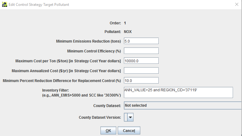
When Least Cost Curve is selected from the Type of Analysis pull-down menu on the Summary tab three constraints settings are available in the Least Cost Curve section of the Constraints tab: Domain-wide Percent Reduction Increment (%): increment for subsequent least cost runs to iterate on until the end percent reduction is reached. Domain-wide Percent Reduction Start (%): target emissions reduction for the first least cost run; and Domain-wide Percent Reduction End (%): final emissions reduction target of the emissions reductions for the incremental least cost runs.
The Least Cost Curve strategy uses all three constraints in an iterative control run. First it will run the least cost strategy with the percent reduction specified as the value of Domain-wide Percent Reduction Start (%). It will then add the Domain-wide Percent Reduction Increment (%) to the starting percent value and will run the least cost strategy at that value (i.e., starting value + increment). It will continue running strategies for each increment until it reaches the value of Domain-wide Percent Reduction End (%). Note that it may not be possible to achieve some of the selected percent reductions, in which case CoST will generate the same result for that increment as the Maximum Emissions Reduction control strategy run would generate.
The Multi-Pollutant Maximum Emissions Reduction control strategy type presents a different Constraints Tab than the other control strategy types. Since this strategy type is running goals on numerous target pollutants (e.g. PM2.5-PRI, NOx, SO2), the constraints presented in Table 4.7 are combined with an inventory filtering capability (see Inputs on the Inventories Tab) to allow for pollutant-specific constraints. The Multi-Pollutant control strategy Constraints tab interface is shown in Figure 4.16.
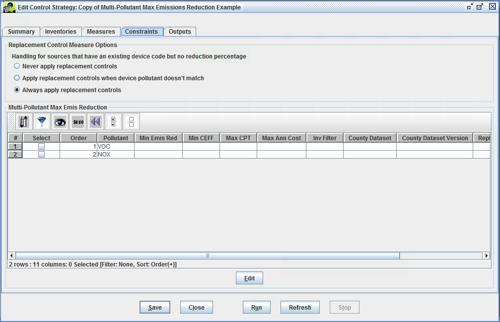
The first step in configuring a Multi-Pollutant Maximum Emissions Reduction control strategy is to select the target pollutants from the Target Pollutant list on the Summary tab. The pollutants selected from this list will appear in the table on the Constraints tab. Note that the order the pollutants are added to the Target Pollutant list is important because it sets the order by which controls are applied in the multi-pollutant strategy.
To set the constraints and filters for each pollutant, click the checkbox in the Select column next to a pollutant on the Constraints tab and click Edit. The Edit Control Strategy Target Pollutant window will appear for setting the constraints and filters to use as the control strategy for the selected pollutant. Figure 4.17 shows an example Edit Control Strategy Target Pollutant window. The fields in the Edit Control Strategy Window include:
Minimum Emissions Reduction(tons): sets the minimum emissions reduction tonnage for a particular source (down to the plant+point+stack+segment level of specification); only control measures that meet this threshold will be considered for the strategyMinimum Control Efficiency(%): requires that control measures used in the strategy have a control efficiency greater than or equal to the specified percentage for a particular source and target pollutantMaximum 2013 Cost per Ton($/ton): requires that control measures used in the strategy have an annualized cost per ton less than or equal to the specified maximum annualized cost per ton for the target pollutant for each source. This cost is based on 2013 dollarsMaximum 2013 Annualized Cost($/yr): requires that control measures used in the strategy have an annualized cost less than or equal to the specified annualized cost for each source and target pollutant. This cost is based on 2013 dollarsMinimum Percent Reduction Difference for Replacement Control(%): requires that control measures used in the strategy have a percent reduction of emissions that is greater than or equal to the specified difference in order for an old control measure to be “replaced by” the new control measureInventory Filter: sets a general filter that can be entered using the same syntax as a Structured Query Language (SQL) “where clause.” Any of the columns in the inventory can be used in the expression. Examples include: SCC LIKE '212%' to limit the analysis to apply only to inventory records for which the SCC code starts with 212, and REGION_CD LIKE '06%' OR REGION_CD LIKE '07%' to limit the strategy analysis to apply only to inventory records with FIPS numeric state-county codes starting with 06 or 07.County Dataset/Version: sets an EMF dataset and version with a list of counties to which control measures will apply during the strategy run. Control measures will be applied only to counties that are included in this list. The County Dataset pull-down menu will show the names of the available CSV datasets in the EMF that have the dataset type ‘List of Counties (CSV)’See Table 4.7 for an additional description of how these fields are applied in a control strategy.

Step 5-1: Run Least Cost Example Strategy. After setting all of the example strategy inputs and constraints, as described in Inputs to Control Strategies, click the Run button in the Edit Control Strategy window to start running the strategy. If the strategy was not saved before clicking Run, the changes will automatically be saved to the database. Note if the Edit Control Strategy window for the “Least Cost 2017 NOx Example” strategy is closed, it can be reopened by selecting the strategy from the list of strategies in the Control Strategy Manager and clicking the Edit button.
Step 5-2: Monitor a Control Strategy Run Status. After starting a control strategy run, check the Status window near the bottom of the EMF GUI to view messages about the run. If all inputs have been properly specified, the status message should show “Started running control strategy: your strategy name”. Click the Refresh button on the Status window to see immediate status updates; the Status window will autoupdate every 1-2 minutes.
If the strategy runs successfully, one message will be displayed for each inventory that completes, such as “Completed processing control strategy input dataset: dataset_name.” When the entire run has finished, the following message will be displayed: “Completed running control strategy: your strategy name” in the Status window. Otherwise, message will display stating that the strategy failed with information about why it failed.
Step 5-3: List Control Strategy Run Outputs. Once the strategy run completes, click on the Outputs tab in the Edit Control Strategy window and then click Refresh at the bottom of the window to see the outputs from the run listed in the Output Datasets table (Figure 4.18 and Figure 4.19).
CoST automatically generates three main outputs for successful strategy runs: Strategy Detailed Result, Strategy Measure Summary, and Strategy County Summary. Some strategy types also generate a Strategy Messages output. Least Cost and Least Cost Curve strategies generate a Least Cost Control Measure Worksheet that lists all of the available control measure options for each source in the inventories.
For all types of strategies, CoST can generate a Controlled Inventory on-demand for any of the Strategy Detailed Result datasets. The types of outputs are discussed in more detail in Outputs of Control Strategies. Note that the output datasets are given unique names that include a timestamp indicating when the strategy was run, including the year, month, day, hour, and minute of the run. A description of how to rename output datasets is provided below.
For additional details on the algorithms that are applied to assign measures to sources as part of a strategy run (other than the descriptions in Introduction to Control Strategies), please see the Control Strategy Tool (CoST) Equations Document.
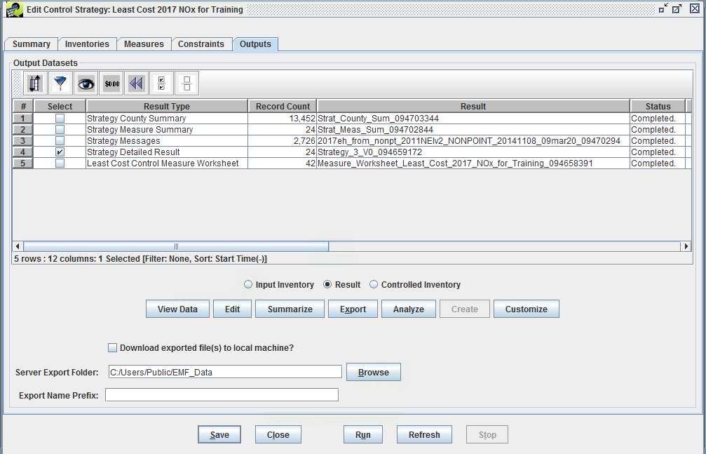
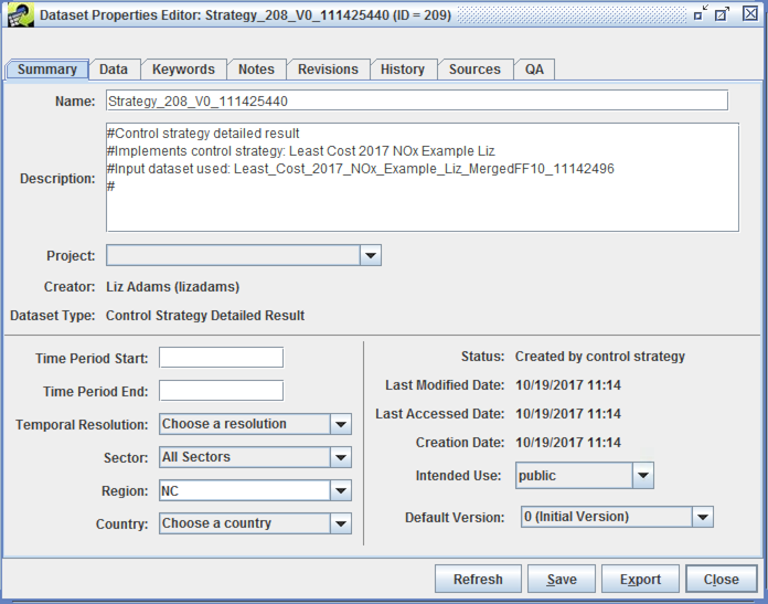
It is possible to perform a number of operations on the strategy outputs. These operations are described in this subsection and the following subsections.
Step 5-4: View Control Strategy Run Outputs. The most basic operation is to view the data of the output dataset using the Data Viewer. To do this, select one of the outputs on the Outputs tab, such as the Strategy Detailed Result, and then click View Data. (Note that the Strategy Detailed Result is the main output on which the Strategy County Summary and Strategy Measure Summary are based.) This will bring up the Data Viewer showing the contents of the Strategy Detailed Result (Figure 4.20).
The Strategy Detailed Result shows the abbreviation of the measure matched to each of the sources for all of the controlled sources, along with columns that identify each controlled source, information about the cost of applying the measures to the sources and the emissions reductions that resulted. The information computed includes the cost of application and the emissions reduced as a result. Enter a sort order (e.g., annual_cost desc) to have the rows sorted in a particular way.
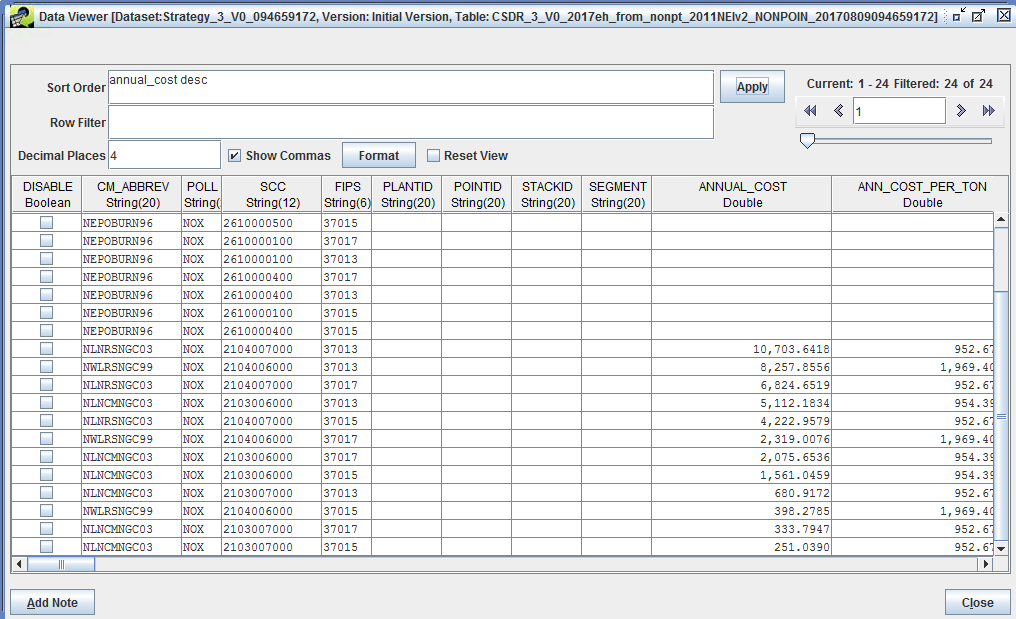
Clear the entries in the Sort Order and Row Filter fields on the Data Viewer and click Apply, all of the data records will be presented in the order in which they appear in the database. More information about the columns included in the detailed result is given in Table 4.9, which is discussed later in the section Strategy Detailed Result.
Click Close to exit from the Data Viewer when you are finished reviewing the Strategy Detailed Result.
Step 5-5: View Control Strategy Run Output Properties. From the Edit Control Strategy Outputs tab, access the properties (metadata) of an output dataset (as opposed to the actual data contained in the output), by selecting an output (for this exercise, select the Strategy Detailed Result) on the Outputs tab of the Edit Control Strategy window and clicking the Edit button. This will bring up the Dataset Properties Editor for the output dataset (Figure 4.21).
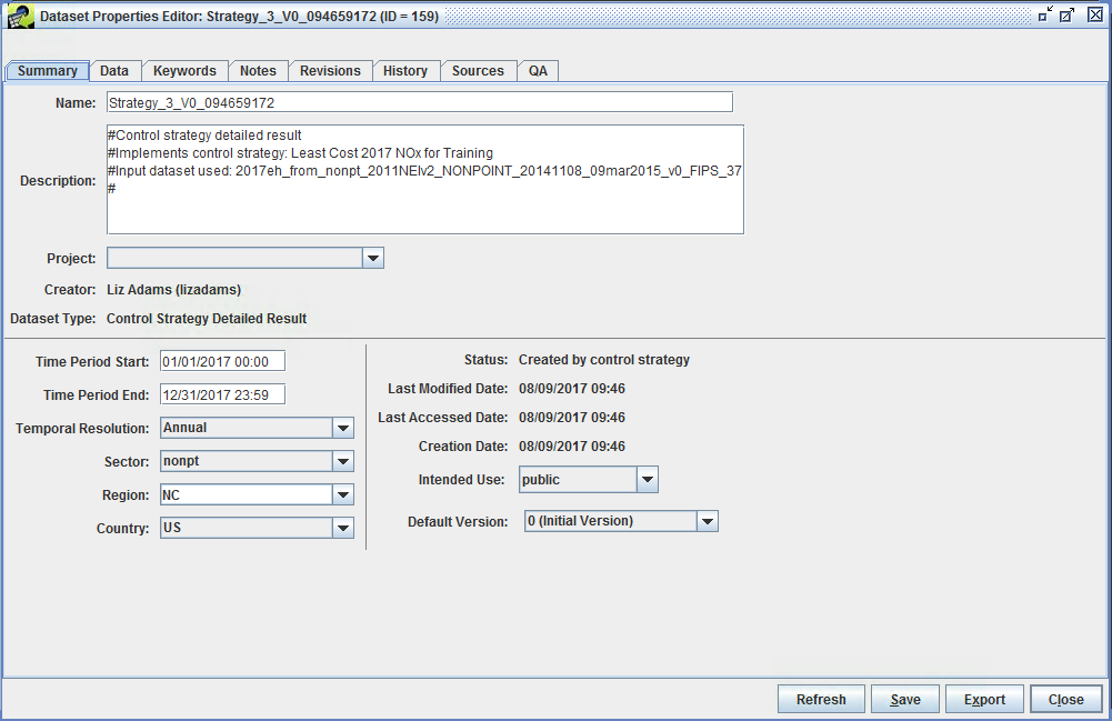
Notice that the tabs on the Dataset Properties Editor are the same as those on the Dataset Properties Viewer shown in Figure 4.10. Editor mode allows many of the fields to be changed, where they could not be changed directly from in the Viewer mode. For example, change the name of the output by replacing the automatically generated name with a more meaningful one (e.g., Least Cost 2017 VOC for Training Result) and then click Save. Notice that unsaved edits are denoted with an asterisk in the title bar of the window.
Examine the other tabs of the Dataset Properties Editor for the Strategy Detailed Result output. In particular see the Keywords tab, an example of which is shown in Figure 4.22. For the Strategy Detailed Result, there are a number of keywords set in the Keywords Specific to Dataset section (in the lower part of window). These keywords correspond to the major parameters of the control strategy, such as the COST_YEAR and the STRATEGY_TYPE as shown in Figure 4.22). There are also keywords for the UNCONTROLLED_EMISSIONS, the TOTAL_EMISSION_REDUCTION, and the ACTUAL_PERCENT_REDUCTION.
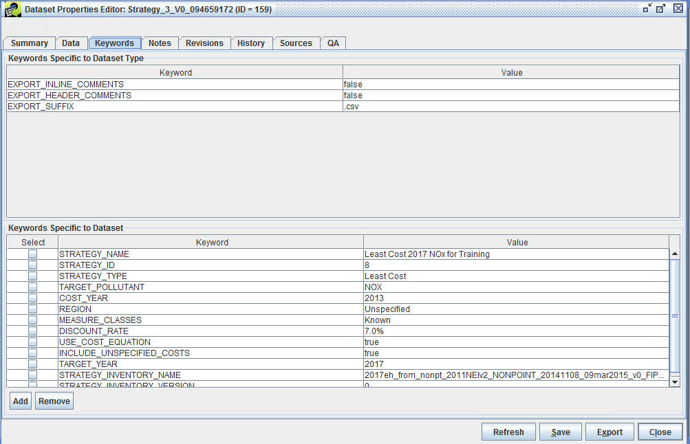
The keywords in the Keywords Specific to Dataset Type section (the upper part of window in Figure 4.22) typically contain directives on how to export the data or other data values that are the same for all datasets of the same type. Typically FF10 or ORL inventories will have some of these keywords.
Note that when the Dataset Properties Editor is open for a dataset no other users can edit that dataset. Similarly, if a control strategy or control measure is open for editing, no other users can edit those items. Users will be able to view these items if the access permissions are set appropriately (see Intended Use setting on the Summary tab).
After examining the other Dataset Properties tabs, close the Dataset Properties Editor by clicking Save to save the changes, or Close to close without saving changes. For the example exercise, click Close and do not save any changes.
Strategy outputs, particularly Strategy Detailed Results, but also the input emissions inventories, can be summarized in many different ways. The ability to prepare summaries is helpful because in many cases there could be thousands of records in a single Strategy Detailed Result or emissions inventory. Thus, when the results of a strategy are analyzed or presented to others, it is useful to show the impact of the strategy in a summarized fashion. Frequently, it is helpful to summarize a strategy for each county, state, SCC, and/or control technology. The summaries are prepared using the EMF subsystem that was originally designed to support quality assurance (QA) of emissions inventories and related datasets, for which summaries are also needed. Thus, each summary is stored as the result of a “QA Step” that is created by having CoST run a SQL query. There are many predefined queries stored in the EMF as ‘templates’, circumventing the need for a user of the system to know SQL to create a summary. Summaries can be added from the QA tab of the Dataset Properties Editor, although there is a shortcut available on the Outputs tab. Summaries are discussed in more detail in Summaries of Strategy Inputs and Outputs.
Step 5-6: Selecting Control Strategy Summaries. Select Strategy Detailed Result on the Outputs tab of the Edit Control Strategy window and then click Summarize to open the QA tab of the Dataset Properties Editor.
To add a new summary from the list of predefined summary templates, click the Add from Template button to see a list of predefined QA Steps (Figure 4.23). To create summaries of interest, click the mouse button on the summaries to create. For this example, select Summarize by Control Technology and Pollutant, Summarize by County and Pollutant, Summarize by Pollutant. Select multiple summaries (as is illustrated in the figure) using Control-Click. Click OK after selecting the summaries and the selected QA templates will be added to the table on the QA tab (Figure 4.24).
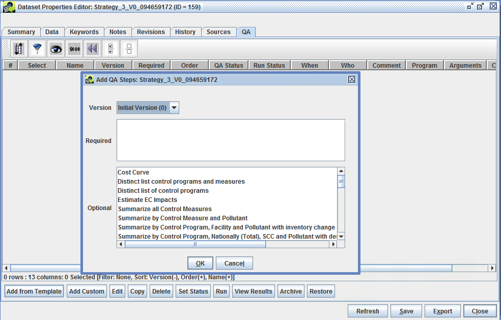
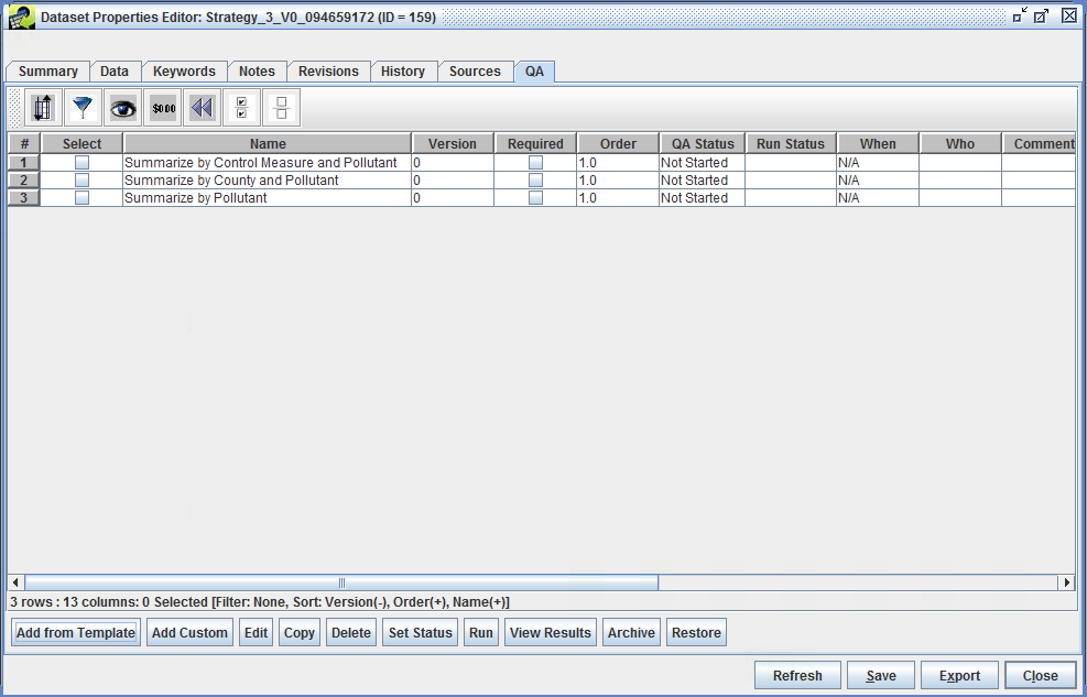
Step 5-7: Running Control Strategy Summaries. To run the QA summaries that are listed on the QA tab, first select the summaries of interest and then click Edit. The Edit QA Step window will appear (Figure 4.25). Do not edit anything in this window, just view the properties of the QA summary. Click Run at the bottom of the window to start the QA summary processing.
Monitor the progress of the QA step in the Status window at the bottom of the EMF main window. Once the run is complete, click the Refresh button to populate the Output Name, Run Status, and Run Date fields in the Edit QA Step window. Note: as an alternative to clicking Run on several different windows, you can instead select a few summaries and click Run on the QA tab.
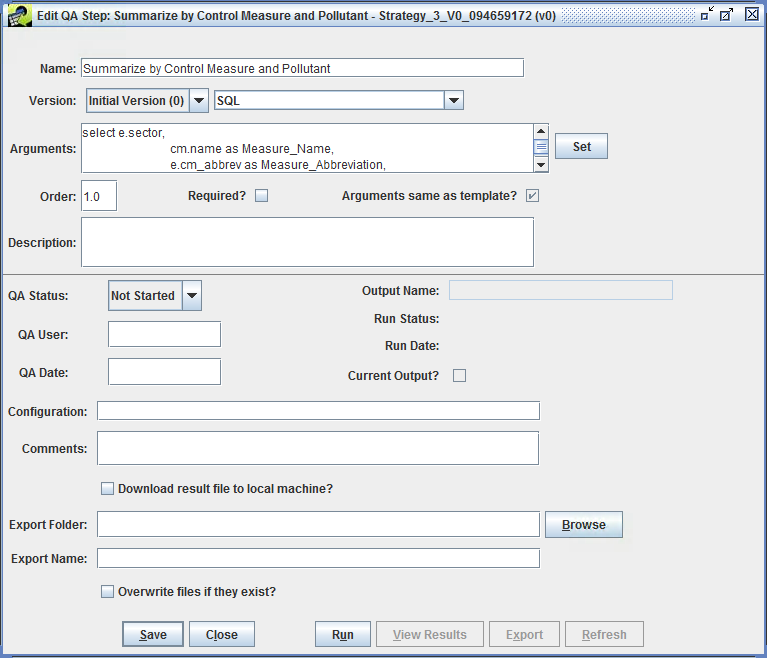
Step 5-8: Viewing Control Strategy Summaries. To see summarized control strategy output, select a checkbox next to the summary of interest on the QA tab and click View Results to bring up the View QA Step Results window (Figure 4.26). Sort and filter the results in this window in the same way as the Control Measure Manager and Control Strategy Manager. For example, click on the avg_cost_per_ton column header to sort on the cost per ton. You can also show the Top n or Bottom n rows using the second and third from the left toolbar buttons. The colorful toolbar buttons on the right support computing statistics, creating plots (if you have the R software package installed on your client machine), and saving the table and plot configurations.
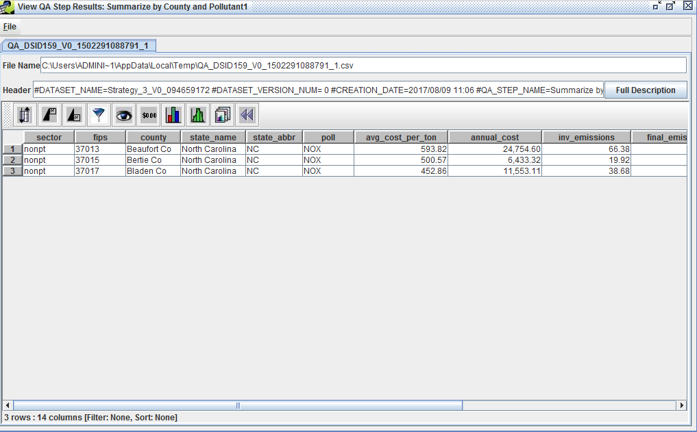
Step 5-9: Export Control Strategy Summary to Google Earth (KMZ). If the summary has longitude and latitude information (e.g., a plant, state, or county summary), the EMF has an interface to create Google Earth-compatible Keyhole Markup Language Zipped (.kmz) files by choosing Google Earth from the File menu of the View QA Step Results window. The interface to create these files is shown in Figure 4.27. Note that the following detailed result summaries have longitude and latitude:
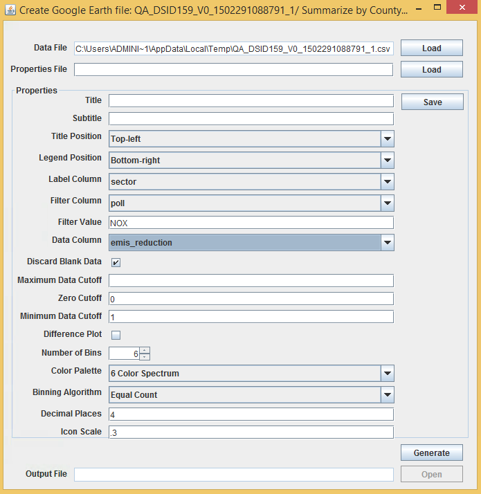
In the Create Google Earth file window, select a Label Column that will be used to label the points in the .kmz file. This label will appear when hovering over a point in the Google Earth map. For a plant summary this would typically be plant_name, for a county summary this would be county, and for a state summary, this would be state_name.
Select a Data Column to show the value of a point in the .kmz file. This value will appear when hovering over a point in the Google Earth map. (e.g., total_emissions_reduction, total_annual_cost, or avg_cost_per_ton). The mouse over information will have the form:
value from Label column : value from Data Column.
For a summary that includes multiple pollutants, specify a filter so that data for only one pollutant is included in the .kmz file. Set the Filter Column to poll (e.g., pollutant), and then specify a Filter Value for a specific inventory pollutant (e.g., NOX).
Use Minimum Data Cutoff to limit the points shown in the .kmz file to include only those that reach a certain size threshold (e.g., do not show small sources or sources with a small amount of reduction). Points will only be created for rows in the summary for which the value in the data column exceeds the value given set by Minimum Data Cutoff. For example, if the Data Column is set to total_emissions_reduction, you might enter 1.0 as the Minimum Data Cutoff to show only plants with at least 1 ton of reduction.
Use Icon Scale to control the size of the points displayed in the Google Earth map. The setting of Icon Scale is a real number between 0 and 1. Smaller values produce smaller circles and larger values produce larger circles.
Mouse over the fields in this window to see tooltips with information about the field. After specifying the settings (aside from the Properties file) click Generate to create the .kmz file using default file name. The name and location of the output file are set by the Output File field.
Click Save to save the settings of the Google Earth file Properties to a file. Load a saved set of properties using the Load button in the Create Google Earth file window.
Close the Create Google Earth file window by clicking the X at the top right corner.
Step 5-10: Export Control Strategy Summaries to CSV. From the Edit QA Step window (Figure 4.25) select a folder to export the results by either typing a directory path in the Export Folder field, or by using the Browse button to select an output directory. Click the Export button and the Export QA Step Result will be written to the selected folder on the EMF server.
Return to the Outputs tab of the Edit Control Strategy window (Figure 4.18).
Step 5-11: Export Control Strategy Outputs. To export the strategy output datasets to the EMF server, enter a folder/directory name into the Server Export Folder field on the Outputs tab. Use the checkboxes to select one or more results files to export from the Output Datasets table and click Export. The files will be written as ASCII files to the Server Export Folder. The resulting CSV files can be imported into a spreadsheet or other database software for analysis. Note that the dataset must be exported to a location where the EMF application user has read/write access to the folder (e.g., the same directory as specified in the environment variable, EMF_DATA_DIRECTORY, in the EMF installation batch file).
It is possible to view the strategy results directly from the Outputs tab in a sortable, filterable table, similar to the table used by the View QA Step Results window (Figure 4.26).
Step 5-12: Analyze Control Strategy Outputs in CoST. Use the checkboxes to select one or more results files to analyze from the Output Datasets table and click Analyze to show the Analyze Control Strategy window for the selected outputs. An example of a Strategy County Summary analysis is shown in Figure 4.28. The results in this window can be sorted, filtered, plotted, and summarized with statistics. An example of a Least Cost Curve Summary is shown in Figure 4.29. Exit from the Analyze Control Strategy window using the X at the top of the window.
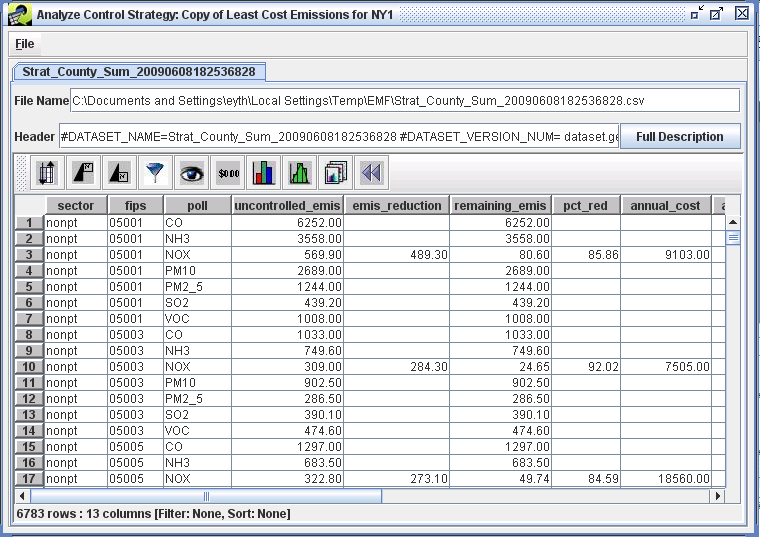
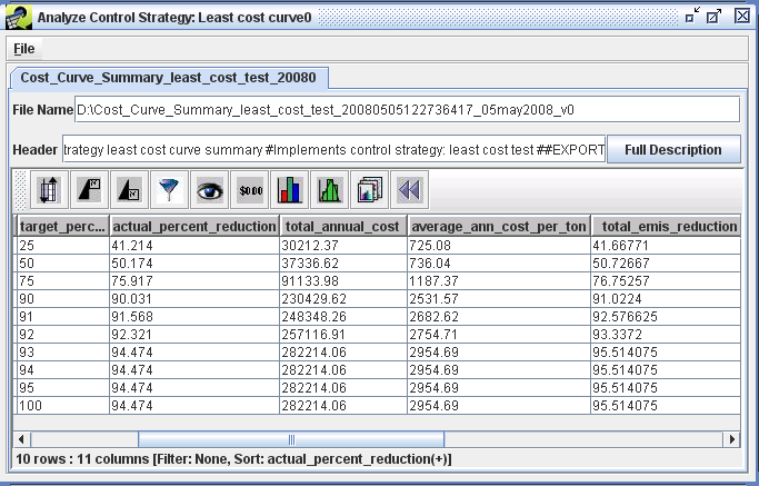
CoST can create a controlled emissions inventory that reflects the effects of the control strategy by merging the detailed result with the original emissions inventory. Details on controlled inventories are discussed further in the section Controlled Emissions Inventory.
Step 5-13: Creating a Controlled Inventory. To create a controlled inventory, click the Controlled Inventory radio button on the Outputs tab of the Edit Control Strategy window (Figure 4.18) and select the Strategy Detailed Result in the Output Datasets table to enable the Create button. Note that only creators of a strategy or the Administrator can create inventories from a strategy result.
Click Create to receive a prompt to Enter a name prefix for the controlled inventories; for this exercise, enter training and click the OK button. Cancelling this prompt will result in a controlled inventory with no name prefix. The status of the inventory creation will be shown in the Status window. Once the controlled inventory has been successfully created, for all but the Least Cost control strategy types the name of the inventory will appear at the far right of the Output Datasets table in the row corresponding to the Strategy Detailed Result. For Least Cost control strategy types, the controlled inventory will show up as rows in the Output Datasets table under the “Controlled Inventory” Result Type. Figure 4.30 shows an example of where the controlled inventory name is located for a Maximum Emissions Reduction control strategy. Figure 4.31 shows an example of where the controlled inventories are located for a Least Cost control strategy.
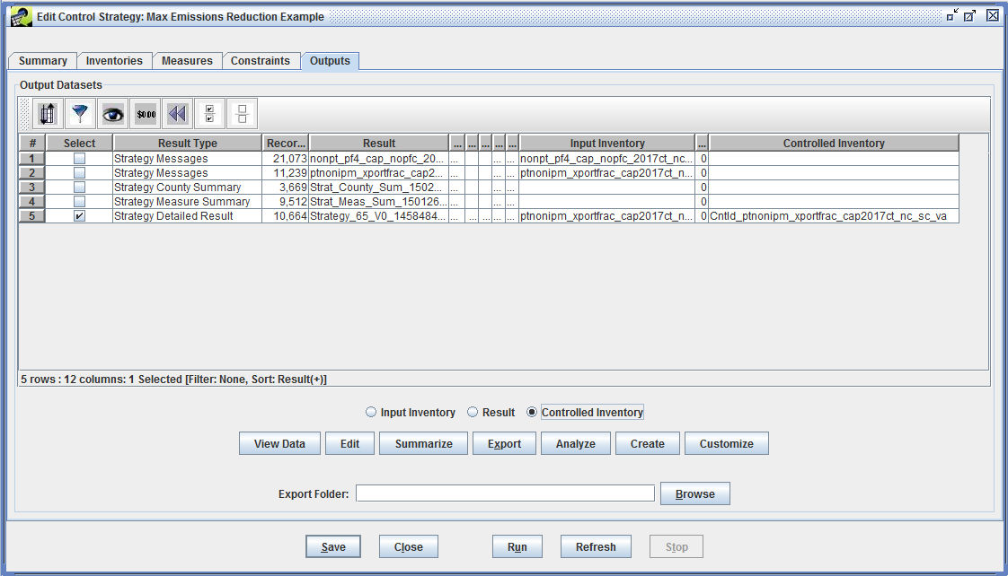
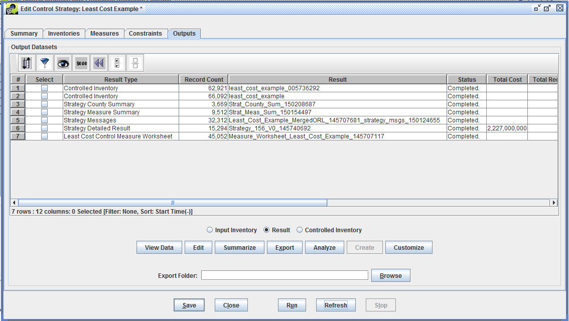
Step 5-14: Viewing a Controlled Inventory. To view the data for a controlled inventory generated from all but the Least Cost control strategy types, select the Controlled Inventory radio button and click View Data (Figure 4.30). For Least Cost control strategy types use the checkbox in the Select column of the Output Datasets table to select a controlled inventory, select the Result radio button, and click View Data (Figure 4.31). The data for the controlled inventory dataset will appear in the Data Viewer.
To view the data for the input inventory that was merged with the Strategy Detailed Result to create the controlled inventory, select the Input Inventory radio button and click View Data.
The Customize button on the Outputs tab is not frequently used, but can generate special types of outputs related to analyses with a Response Surface Model (RSM). These custom outputs are not discussed here.
The remainder of this chapter provides reference documentation on the outputs of strategies and summaries that can be created with CoST. Additional advanced exercises and examples are available in Chapter 5.
This section provides details on the contents of each type of CoST output.
As noted earlier, the Strategy Detailed Result is the primary output from running a control strategy. It is a table of emission source-control measure pairings, each of which contains information about the costs and emission reduction achieved for measures after they are applied to the sources. The contents of this table are described later in this subsection. When generating the Strategy Detailed Result table, some data are needed for CoST to calculate the values of some columns related to costs, such as:
Capital to Annual Ratio: from the control measure efficiency recordInterest Rate: from the control strategyEquipment Life (yrs): from the control measure efficiency recordStack Flow Rate (cfs): from the emissions inventoryBoiler Capacity (MW): from the design capacity column of the inventory; units are obtained from the design_capacity_unit_numerator and design_capacity_unit_denominator columns from the inventory. Note that boiler capacity is often blank in inventories, so special steps may need to be taken to fill in this information.The capital to annual ratio is used to calculate the capital costs of a control device from an available O&M cost estimate for that device. The capital costs are the one-time costs to purchase and install the device, while the operating and maintenance (O&M) costs are those required to operate and maintain the device for each year. The interest rate and equipment life are used to compute the annualized capital costs for the device. The interest rate is an annual interest rate used to calculate the cost of borrowing money to purchase and install the control device. The annualized capital cost is computed based on the interest rate, and the costs are spread over the life of the equipment. The algorithms to compute these cost breakdowns vary based on whether the input data required to use a cost equation are available. This topic is described in further detail in Table 4.9, which is given after an introductory discussion of cost concepts, below. The columns of the Strategy Detailed Result are also given in Table 4.9.
When cost data are provided for the control measures, the resulting costs are also specified in terms of a particular year. To compute the cost results for a control strategy, it is necessary to escalate or de-escalate the costs to the same year in order to adjust for inflation and to allow for consistency in comparing control strategy results. This is done with the following formula:
Cost ($) for a year of interest = (Cost for original cost year x GDP IPD for year of interest) / GDP IPD for original cost year
where the GDP IPD is the Gross Domestic Product Implicit Price Deflator.
Implicit Price Deflator (IPD) values are available from the United States Department of Commerce Bureau of Economic Analysis Table 1.1.9. Implicit Price Deflators for Gross Domestic Product. The current version used is from March 2018. An excerpt of this version is shown in Table 4.8.
| Year | GDP IPD | Year | GDP IPD | Year | GDP IPD | Year | GDP IPD | |||
|---|---|---|---|---|---|---|---|---|---|---|
| 1980 | 44.377 | 1990 | 66.773 | 2000 | 81.887 | 2010 | 101.221 | |||
| 1981 | 48.520 | 1991 | 68.996 | 2001 | 83.754 | 2011 | 103.311 | |||
| 1982 | 51.530 | 1992 | 70.569 | 2002 | 85.039 | 2012 | 105.214 | |||
| 1983 | 53.565 | 1993 | 72.248 | 2003 | 86.735 | 2013 | 106.913 | |||
| 1984 | 55.466 | 1994 | 73.785 | 2004 | 89.120 | 2014 | 108.832 | |||
| 1985 | 57.240 | 1995 | 75.324 | 2005 | 91.988 | 2015 | 110.012 | |||
| 1986 | 58.395 | 1996 | 76.699 | 2006 | 94.814 | 2016 | 111.416 | |||
| 1987 | 59.885 | 1997 | 78.012 | 2007 | 97.337 | 2017 | 113.421 | |||
| 1988 | 61.982 | 1998 | 78.859 | 2008 | 99.246 | |||||
| 1989 | 64.392 | 1999 | 80.065 | 2009 | 100 |
To facilitate the comparison of the costs of control measures with one another, a normalized version of the control measure cost per ton is stored within the control measures database. These costs have all been converted to a consistent “reference year” using the above formula, so that the cost of any measure can be compared with any other even if their cost years differ. Currently, the reference year is 2013. In addition, during the course of the strategy run, the costs are converted (using the above formula) from the reference year to the cost year that was specified as an input to the strategy. The results of the strategy are therefore presented in terms of the specified cost year.
As indicated above, Table 4.9 provides details on the columns of the Strategy Detailed Result.
| Column | Description |
|---|---|
| DISABLE | A true-false value that determines whether to disable the control represented on this line during the creation of a controlled inventory. |
| CM_ABBREV | The abbreviation for the control measure that was applied to the source. |
| POLL | The pollutant for the source, found in the inventory. |
| SCC | The SCC for the source, found in the inventory. |
| REGION_CD | The state and county FIPS code for the source, found in the inventory. |
| FACILITY_ID | For point sources, the facility ID for the source from the inventory. |
| UNIT_ID | For point sources, the unit ID for the source from the inventory. |
| REL_POINT_ID | For point sources, the release point ID for the source from the inventory. |
| PROCESS_ID | For point sources, the process ID for the source from the inventory. |
| ANNUAL_COST ($) | The total annual cost (including both capital and O&M) required to keep the measure on the source for a year. Default Approach (used when there is no cost equation, or when inputs to cost equation are not available): Annual Cost = Control Emissions Reduction (tons) x Reference Yr CPT ($/tons in 2013 Dollars) x Cost Yr GDP IPD / Reference Yr GDP IPD |
| CTL_ANN_COST_PER_TON ($/ton) | The annual cost (both capital and O&M) to reduce one ton of the pollutant. Control Annual CPT = Annual Cost ($) / Control Emissions Reduction (tons) |
| EFF_ANN_COST_PER_TON ($/ton) | The effective annual cost (both capital and O&M) to reduce one ton of the pollutant. Effective Annual CPT = Annual Cost ($) / Effective Emissions Reductions (tons) |
| ANNUAL_OPER_MAINT_COST ($) | The annual cost to operate and maintain the measure once it has been installed on the source. Default Approach (used when there is no cost equation, or inputs to cost equation are not available): Annual O&M Cost = Annual Cost - Annualized Capital Cost |
| ANNUAL_VARIABLE_OPER_ |
The annual variable cost to operate and maintain the measure once it has been installed on the source. Only calculated when using a cost equation that specifies this cost. |
| ANNUAL_FIXED_OPER_MAINT_ |
The annual fixed cost to operate and maintain the measure once it has been installed on the source. Only calculated when using a cost equation that specifies this cost. |
| ANNUALIZED_CAPITAL_COST ($) | The annualized cost of installing the measure on the source assuming a particular interest rate and equipment life. Annualized Capital Cost = Total Capital Cost x Capital Recovery Factor (CRF) Note: if the CRF can not be calculated for the measure, it is not possible to compute the annualized capital cost or the breakdown of costs between capital and O&M costs. CRF = (Interest Rate x (1 + Interest Rate)^Equipment Life) / ((Interest Rate + 1) ^Equipment Life - 1) |
| TOTAL_CAPITAL_COST ($) | The total cost to install a measure on a source. Default Approach (used when there is no cost equation or cost equation inputs are not available): Total Capital Cost = Annual Cost ($) x Capital to Annual Ratio |
| CONTROL_EFF (%) | The control efficiency of the measure being applied, stored in the measure efficiency record. |
| RULE_PEN (%) | The rule penetration of the measure being applied, stored in the measure efficiency record, but could be overridden as a strategy setting (see Inputs on the Measures Tab). |
| RULE_EFF (%) | The rule effectiveness of the measure being applied, stored in the measure efficiency record, but could be overridden as a strategy setting (see Inputs on the Measures Tab). |
| PERCENT_REDUCTION (%) | The percent by which the emissions from the source are reduced after the control measure has been applied. Percent Reduction = Control Efficiency (%) x Rule Penetration (%) x Rule Effectiveness (%) |
| ADJ_FACTOR | The factor that was applied by a control program to adjust the emissions to the target year. Only appicable to the “Project Future Year Inventory” strategy type. |
| INV_CTRL_EFF (%) | The control efficiency for the existing measure on the source (if any), found in the emissions inventory. Used to calculate uncontrolled annual emissions. |
| INV_RULE_PEN (%) | The rule penetration for the existing measure on the source (if any), found in the emissions inventory. Used to calculate uncontrolled annual emissions. |
| INV_RULE_EFF (%) | The rule effectiveness for the existing measure on the source (if any), found in the emissions inventory. Used to calculate uncontrolled annual emissions. |
| FINAL_EMISSIONS (tons) | The final emissions that result from the source being controlled. Final Emissions = Inventory Annual Emissions (tons) - Effective Emissions Reductions (tons) |
| CTL_EMIS_REDUCTION (tons) | The emissions reduction (in tons) as a result of applying the control measure to the source. Control Emissions Reduction = Uncontrolled Annual Emissions (tons) x Percent Reduction (%) |
| EFF_EMIS_REDUCTION (tons) | The effective emissions reduction (in tons) as a result of applying the control measure to the source, taking into account the reduction achieved by the existing control (if any). Effective Emissions Reduction = Control Emissions Reduction - (Uncontrolled Annual Emissions - Inventory Annual Emissions) |
| INV_EMISSIONS (tons) | The annual emissions, found in the emissions inventory. Note that if the starting inventory had average-day emissions, the average-day value is annualized and the resulting value is shown here. This is necessary to properly compute the costs of the measure. |
| APPLY_ORDER | If multiple measures are applied to the same source, this is a numeric value noting the order of application for this specific control measure. The first control to be applied will have a value of 1 for this field, the second will have a value of 2, and so on. |
| INPUT_EMIS (tons) | The INV_EMISSIONS value with any existing control measure removed, i.e. uncontrolled annual emissions. Uncontrolled Annual Emissions = Inventory Annual Emissions / (1 - (Inv. Ctrl. Eff x Inv. Rule Pen. x Inv. Rule Eff.)) |
| OUTPUT_EMIS (tons) | The emissions that still exist for the source after the control measure has been applied. |
| FIPSST | The two-digit FIPS state code. |
| FIPSCTY | The three-digit FIPS county code. |
| SIC | The Standard Industrial Classification (SIC) code for the source from the emissions inventory. |
| NAICS | The North American Industry Classification System (NAICS) code for the source from the emissions inventory. |
| SOURCE_ID | The record number from the input inventory for this source. |
| INPUT_DS_ID | The numeric ID of the input inventory dataset (for bookkeeping purposes). If multiple inventories were merged to create the inventory (as can be done for Least Cost control strategies), this ID is that of the merged inventory. |
| CS_ID | The numeric ID of the control strategy. |
| CM_ID | The numeric ID of the control measure. |
| EQUATION_TYPE | The control measure equation that was used during the cost calculations. |
| ORIGINAL_DATASET_ID | The numeric ID of the original input inventory dataset, even if a merged inventory was used for the computation of the strategy, as can be done for Least Cost control strategies. |
| SECTOR | The emissions inventory sector specified for the input inventory (text, not an ID number; e.g., ptnonipm for the point non-IPM sector) |
| CONTROL_PROGRAM | The control program that was applied to produce this record. Only appicable to the “Project Future Year Inventory” strategy type. |
| XLOC | The longitude for the source, found in the emissions inventory for point sources; for nonpoint inventories the county centroid is used. This is useful for mapping purposes. |
| YLOC | The latitude for the source, found in the emissions inventory for point sources; for nonpoint inventories the county centroid is used. This is useful for mapping purposes. |
| FACILITY | The facility name from the emissions inventory (or county name for nonpoint sources). |
| REPLACEMENT_ADDON | Indicates whether the measure was a replacement or an add-on control. A = Add-On Control, R = Replacement Control |
| EXISTING_MEASURE_ |
This column is used when an Add-On Control was applied to a source; it indicates the existing control measure abbreviation that was on the source. |
| EXISTING_PRIMARY_DEVICE_ |
This column is used when an Add-On Control was applied to a source; it indicates the existing control measure primary device type code that was on the source. |
| STRATEGY_NAME | The name of the control strategy that produced the detailed result. |
| CONTROL_TECHNOLOGY | Indicates the control technology of the control measure. |
| SOURCE_GROUP | Indicates the source group of the control measure. |
| COMMENT | Information about this record and how it was produced; this information is either created automatically by the system or entered by the user. |
| RECORD_ID VERSION DELETE_VERSIONS | System specific columns used for tracking primary key and versioning of data |
The Strategy Measure Summary output dataset is a table of emissions reductions and cost values aggregated by the emissions sector (i.e., an emissions inventory sector), state/county FIPS code, SCC, pollutant, and control measure. This table contains information only for sources that were controlled during the strategy run. It is generated by running a SQL statement that aggregates the data from the Strategy Detailed Result according to the five categories just listed. The annual cost and emissions reductions are calculated by summing all costs and emissions reductions for the specified grouping (sector, FIPS, SCC, pollutant, and control measure). The average annual cost per ton is calculated by dividing the total annual costs by the total emissions reductions for each measure. The columns contained in this summary and the formulas used to compute their values are shown in Table 4.10. An example Strategy Measure Summary is shown in Table 4.14.
| Column | Description |
|---|---|
| SECTOR | The emissions inventory sector for the source (e.g., ptnonipm for the point non-IPM sector) |
| REGION_CD | The state and county FIPS code for the source |
| SCC | The SCC for the source |
| POLL | The pollutant for the source |
| CONTROL_MEASURE_ABBREV | The control measure abbreviation |
| CONTROL_MEASURE | The control measure name |
| CONTROL_TECHNOLOGY | The control technology that is used for the measure (e.g., Low NOx burner, Onroad Retrofit). |
| SOURCE_GROUP | The group of sources to which the measure applies (e.g., Fabricated Metal Products - Welding). |
| ANNUAL_COST | The total annual cost for all sources that use this measure. This is calculated by summing all source annual costs that use this measure |
| AVG_ANN_COST_PER_TON | The average annual cost per ton ($/ton). This is calculated by dividing the total annual cost by the total emissions reductions for all sources for this measure |
| INPUT_EMIS | The total of emissions from all sources entering the control measure. This is calculated by summing the input emissions for all sources that were controlled by this measure |
| EMIS_REDUCTION | The total reduction in emissions in tons for all sources for this control measure |
| PCT_RED | The percent reduction (%) for all sources controlled by this measure. This is calculated by dividing the total emissions reductions by the total input emissions. |
| RECORD_ID VERSION DELETE_VERSIONS | System specific columns used for tracking primary key and versioning of data |
The Strategy County Summary output dataset is a table of emissions reductions and cost values aggregated by emissions sector, county, and pollutant. This dataset includes all of the emissions inventory sources regardless of whether they were controlled. If there is more than one inventory included in the control strategy inputs, then all inventories and their associated Strategy Detailed Results are merged and aggregated in this summary. The columns that compose this summary are shown in Table 4.11. An example Strategy County Summary is shown in Table 4.15.
| Column | Description |
|---|---|
| SECTOR | The emissions inventory sector for the source (i.e., ptnonipm for the point non-IPM emissions sector) |
| REGION_CD | The state and county FIPS code for the source |
| POLL | The pollutant for the source |
| UNCONTROLLED_EMIS | The original inventory emissions for the county (in tons) |
| EMIS_REDUCTION | The total emissions reductions for the county (in tons) |
| REMAINING_EMIS | The remaining emissions after being controlled (in tons) |
| PCT_RED | The percent reduction for the pollutant |
| ANNUAL_COST | The total annual cost for the county. This is calculated by summing the annual costs for the county |
| ANNUAL_OPER_MAINT_COST | The total annual O&M costs for the county. This is calculated by summing the annual O&M costs for the county |
| ANNUALIZED_CAPITAL_COST | The total annualized capital costs for the county. This is calculated by summing the annualized capital costs for the county |
| TOTAL_CAPITAL_COST | The total capital costs for the county. This is calculated by summing the total capital costs for the county |
| AVG_ANN_COST_PER_TON | The average annual cost per ton ($/ton). This is calculated by dividing the total annual cost by the total emission reduction for the county. |
| RECORD_ID VERSION DELETE_VERSIONS | System specific columns used for tracking primary key and versioning of data |
Another output that can be created is a controlled emissions inventory (introduced earlier in Creating a Controlled Emissions Inventory). This dataset is not automatically created during a strategy run; instead, a user can choose to create it after the strategy run has completed successfully. When CoST creates a controlled inventory, comments are placed at the top of the inventory file that indicate the strategy that produced it and the high-level settings for that strategy. For the sources that were controlled, CoST fills in the CEFF (control efficiency), REFF (rule effectiveness), and RPEN (rule penetration) columns based on the control measures applied to the sources. It also populates several additional columns toward the end of the ORL inventory rows that specify information about measures that it has applied. These columns are:
CONTROL MEASURES: An ampersand-separated list of control measure abbreviations that correspond to the control measures that have been applied to the given source.PCT REDUCTION: An ampersand-separated list of percent reductions that have been applied to the source, where percent reduction = CEFF x REFF x RPEN.CURRENT COST: The annualized cost for that source for the most recent control strategy that was applied to the source.TOTAL COST: The total cost for the source across all measures that have been applied to the source.In this way, the controlled inventories created by CoST always specify the relevant information about the measures that have been applied as a result of a CoST control strategy.
The Strategy Messages output provides information gathered while the strategy is running that is helpful to the user. The Strategy Messages output is currently created by the following strategy types:
The columns of the Strategy Messages output are described in Table 4.12. An example Strategy Messages output is shown in Table 4.13.
| Column | Description |
|---|---|
| REGION_CD | The state and county FIPS code for the source, found in the emissions inventory |
| SCC | The SCC code for the source, found in the emissions inventory |
| FACILITY_ID | For point sources, the plant ID for the source from the emissions inventory. |
| UNIT_ID | For point sources, the point ID for the source from the emissions inventory. |
| REL_POINT_ID | For point sources, the stack ID for the source from the emissions inventory. |
| PROCESS_ID | For point sources, the segment for the source from the emissions inventory. |
| POLL | The pollutant for the source, found in the emissions inventory |
| STATUS | The status type of the message. The possible values: Warning - a possible issue has been detected, but processing did not stop; Error - a problem occurred that caused the processing to stop; or Informational - it was desirable to communicate information to the user. |
| CONTROL_PROGRAM | The control program for the strategy run; this is populated only when using the “Project Future Year Inventory” strategy type. |
| MESSAGE | Text describing the strategy issue. |
| MESSAGE_TYPE INVENTORY PACKET_REGION_CD PACKET_SCC PACKET_FACILITY_ID PACKET_UNIT_ID PACKET_REL_POINT_ID PACKET_PROCESS_ID PACKET_POLL PACKET_SIC PACKET_MACT PACKET_NAICS PACKET_COMPLIANCE_DATE | Reserved columns used for another strategy type that was not part of this training exercise. |
| RECORD_ID VERSION DELETE_VERSIONS | System specific columns used for tracking primary key and versioning of data |
| region cd | scc | facility id | unit id | rel point id | process id | poll | status | control program | message |
|---|---|---|---|---|---|---|---|---|---|
| 42049 | 30900201 | 420490009 | 942 | S942 | 1 | PM25-PRI | Warning | Negative emission reduction (-1693.9) |
| SECTOR | REGION CD | SCC | POLL | CONTROL MEASURE ABBREV | CONTROL MEASURE | CONTROL TECH. | SOURCE GROUP | ANNUAL COST | AVG ANN COST PER TON | EMIS REDUCTION |
|---|---|---|---|---|---|---|---|---|---|---|
| ptnonipm | 37001 | 10200906 | PM10-PRI | PFFPJIBWD | Fabric Filter (Pulse Jet Type); (PM10) Industrial Boilers - Wood | Fabric Filter (Pulse Jet Type) | Industrial Boilers - Wood | $419,294 | $12,862 | 32.6007 |
| ptnonipm | 37001 | 10200906 | PM25-PRI | PFFPJIBWD | Fabric Filter (Pulse Jet Type); (PM10) Industrial Boilers - Wood | Fabric Filter (Pulse Jet Type) | Industrial Boilers - Wood | 19.5426 | ||
| ptnonipm | 37001 | 30500311 | PM10-PRI | PFFPJMIOR | Fabric Filter (Pulse Jet Type); (PM10) Mineral Products - Other | Fabric Filter (Pulse Jet Type) | Mineral Products - Other | $446,026 | $83,379 | 5.3494 |
| ptnonipm | 37001 | 30500311 | PM25-PRI | PFFPJMIOR | Fabric Filter (Pulse Jet Type); (PM10) Mineral Products - Other | Fabric Filter (Pulse Jet Type) | Mineral Products - Other | 2.0939 | ||
| ptnonipm | 37001 | 30501110 | PM10-PRI | PFFPJMIOR | Fabric Filter (Pulse Jet Type); (PM10) Mineral Products - Other | Fabric Filter (Pulse Jet Type) | Mineral Products - Other | $110 | $147 | 0.7498 |
| ptnonipm | 37001 | 30501110 | PM25-PRI | PFFPJMIOR | Fabric Filter (Pulse Jet Type); (PM10) Mineral Products - Other | Fabric Filter (Pulse Jet Type) | Mineral Products - Other | 0.2605 |
| SECTOR | REGION CD | POLL | INPUT EMIS | EMIS REDUCTION | REMAINING EMIS | PCT RED | ANNUAL COST | ANNUAL OPER MAINT COST | ANNUALIZED CAPITAL COST | TOTAL CAPITAL COST | AVG ANN COST PER TON |
|---|---|---|---|---|---|---|---|---|---|---|---|
| ptnonipm | 37001 | VOC | 313.8724 | 313.8724 | |||||||
| ptnonipm | 37001 | PM25-PRI | 33.4717 | 33.2505 | 0.2212 | 99.3391 | |||||
| ptnonipm | 37001 | NH3 | 6.9128 | 6.9128 | |||||||
| ptnonipm | 37001 | NOX | 146.2904 | 146.2904 | |||||||
| ptnonipm | 37001 | PM10-PRI | 51.0928 | 50.7019 | 0.3909 | 99.2349 | $865,430 | $746,831 | $83,300 | $882,489 | $22,363 |
| ptnonipm | 37001 | SO2 | 54.3864 | 54.3864 |
The EMF/CoST system can prepare summaries of the datasets that are loaded into the system, including both the emissions inventory datasets and the Strategy Detailed Result outputs. The ability to prepare summaries is helpful because in many cases there could be thousands of records in a single Strategy Detailed Result. Thus, when the results of a strategy are analyzed or presented to others, it is useful to show the impact of the strategy in a summarized fashion. Frequently, it is helpful to summarize a strategy for each county, state, SCC, or control technology. The power of the PostgreSQL relational database that contains the system data is used to develop these summaries. Currently, they are prepared using the EMF subsystem that was designed to support quality assurance of emissions inventories and related datasets. Recall that the creation of summaries for strategy outputs was discussed in Summarizing Strategy Outputs.
Each summary is stored as the result of a “QA Step” that is created by asking CoST to run a SQL query. Summaries can be added to inventory or Strategy Detailed Result datasets by editing the dataset properties, going to the QA tab, and using the available buttons to add and edit QA steps. For more details on how to create summaries, see Summarizing Strategy Outputs. Examples of the types of summary templates available for Point Source Inventories (the type with the most templates due to the larger number of columns in that inventory type) are:
Note that the summaries “with Descriptions” have more information than the ones without. For example, the “Summarize by SCC and Pollutant with Descriptions” summary includes the SCC description in addition to the pollutant description. The disadvantage to include the descriptions is that they are a bit slower to generate because information has to be brought in from additional tables than just the table being summarized.
Each of the summaries is created using a customized SQL syntax that is very similar to standard SQL, except that it includes some EMF-specific concepts that allow the queries to be defined generally and then applied to specific datasets as needed. An example of the customized syntax for the “Summarize by SCC and Pollutant” query is:
Notice that the only difference between this and standard SQL is the use of the $TABLE[1] syntax. When this query is run, the $TABLE[1] portion of the query is replaced with the table name used to contain the data in the EMF. Note that most datasets have their own tables in the EMF schema, so you do not normally need to worry about selecting only the records for the specific dataset of interest. The customized syntax also has extensions to refer to another dataset and to refer to specific versions of other datasets using tokens other than $TABLE. For the purposes of this discussion, it is sufficient to note that these other extensions exist.
Some of the summaries are constructed using more complex queries that join information from other tables, such as the SCC descriptions, the pollutant descriptions (which are particularly useful for HAPs), and to account for any missing descriptions. For example, the syntax for the “Summarize by SCC and Pollutant with Descriptions” query is:
select e.SCC,
 coalesce(s.scc_description,'AN UNSPECIFIED DESCRIPTION')::character varying(248)
 as scc_description, e.POLL,
 coalesce(p.descrptn,'AN UNSPECIFIED DESCRIPTION')::character varying(11)
 as pollutant_code_desc,
 coalesce(p.name,'AN UNSPECIFIED SMOKE NAME')::character varying(11)
 as smoke_name, p.factor, p.voctog, p.species,
 coalesce(sum(ann_emis), 0) as ann_emis, coalesce(sum(avd_emis), 0) as avd_emis
from $TABLE[1] e
left outer join reference.invtable p on e.POLL=p.cas
left outer join reference.scc s on e.SCC=s.scc
group by e.SCC,e.POLL,p.descrptn,s.scc_description,
 p.name, p.factor,p.voctog, p.species
order by e.SCC, p.name
This query is quite a bit more complex, but is still supported by the EMF QA step processing system. In addition to summaries of the inventories, there are many summaries available for the Strategy Detailed Results output by control strategy runs and for some of the other CoST-related dataset types. Some of the summaries available for Strategy Detailed Results are as follows:
A plot created based on the output of a Summarize by Control Technology and Pollutant summary is shown in Figure 4.32.
When multiple datasets need to be considered in a summary (e.g., to compare two emissions inventories), the EMF “QA Program” mechanism is used. The QA programs each have customized user interfaces that allow users to select the datasets to be used in the query. Some of the following QA programs may prove useful to CoST users:
Multi-inventory sum: takes multiple inventories as input and reports the sum of emissions from all inventoriesMulti-inventory column report: takes multiple inventories as input and shows the emissions from each inventory in separate columnsMulti-inventory difference report: takes two sets of inventories as input, sums each inventory, and then computes the difference between the two sumsCompare Control Strategies: compares the data available in the Strategy Detailed Result datasets output from two control strategiesSummaries can be mapped with geographic information systems (GIS), mapping tools, and Google Earth. To facilitate this mapping, many of the summaries that have “with Descriptions” in their names include latitude and longitude information. For plant-level summaries, the latitude and longitude provided are the average of all the values given for the specific combination of FIPS and PLANT_ID. For county- and state-level summaries, the latitude and longitude are the centroid of the county or state specified in the fips table of the EMF reference schema.
It is useful to note that after the summaries have been created, they can be exported to CSV files. By clicking View Results, the summary results can be viewed in a table called the Analysis Engine that does sorting, filtering, and plotting. From the File menu of the Analysis Engine window, a compressed .kmz file can be created and subsequently loaded into Google Earth. Note that each KMZ file is currently provided with a single latitude and longitude coordinate representing its centroid, even for geographic shapes like counties.
Recall that in addition to the datasets output for control strategies, many types of summaries of these datasets can be created in CoST. Figure 4.32 shows a plot summarizing a Least Cost Strategy Detailed Result using the “Summarize by Control Technology and Pollutant” query. Some of the technologies used in this run were Low NOx burners (LNB), Low NOx burners with Flue Gas Recovery (LNB + FGD), Non-Selective Catalytic Reduction (NSCR), and Selective Non-catalytic Reduction (SNCR). Note that Figure 4.32 was generated by plotting data output from CoST with spreadsheet software, and not by CoST itself. CoST does have some plotting capabilities, but they are not discussed in this document.
This chapter includes advanced exercises for learning how to use different features of CoST. Users should complete the exercises in Chapter 3 and Chapter 4 before attempting the exercises in this chapter.
Datasets from the Manage menu of the main EMF window.In many cases, it will be necessary to import an emissions inventory into the EMF for use with CoST. Before it can be imported, the inventory must be in one of these FF10 or ORL formats: Point, Onroad, Nonroad, or Nonpoint. For more information on these formats, see https://www.cmascenter.org/smoke/documentation/4.5/html/ch08s02.html#sect_input_inventory_format. Try importing an inventory using the following steps:
Select an inventory format from Show Datasets of Type menu to the type that represents the inventory to import (e.g., FF10 Nonpoint Inventory).
Click the Import button to show the Import Datasets window.
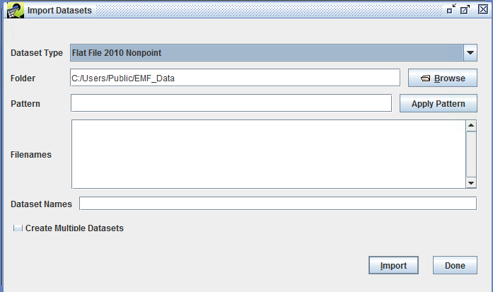
Browse button and browse to the location of the inventory to import on the EMF server computer (e.g., C:\Users\Public\EMF_Data\inventories).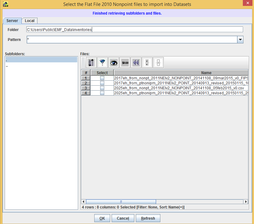
Select the checkbox that corresponds to the inventory (e.g., 2017eh_from_nonpt_2011NEIv2_NONPOINT_20141108_09mar2015_v0_FIPS_37.csv) and then click OK.
Specify a unique, descriptive name for the new dataset in the Dataset Name dialog box.
Click the Import button. Monitor the Status window for the status of the import.
Click Done on the Import Datasets window.
After the Status window messages indicates that the import has completed, click Refresh on the Dataset Manager to see the newly imported inventory dataset. The dataset could now be used as an input to a control strategy.
To import a list of counties to limit the counties used for a strategy analysis, set the Show Datasets of Type menu to List of Counties and then import the file following steps 3 through 9 above. Be sure that the list of counties file has at least two columns, with one of them labeled FIPS.
The Dataset Manager includes the following controls:
View opens the Dataset Properties ViewerEdit Properties opens the Dataset Properties EditorEdit Data creates new versions of the datasetRemove removes the datasetImport imports new datasetsExport exports the data to a file on the EMF serverPurge purges datasets that were removed from the systemClose closes the Dataset Manager Window
For this exercise, an existing Least Cost Strategy will be modified to create a Maximum Emissions Reductions strategy.
From the Control Strategy Manager Copy the least cost strategy created in Chapter 4 to a new strategy.
Edit the strategy and set the Type of Analysis to Max Emissions Reduction.
Run the new strategy and answer the following questions once it completes.
Did the Maximum Emissions Reduction strategy run slower or faster than the Least Cost?
How many more emissions reductions were achieved over the 50% level of reduction set in the Least Cost run in Chapter 4?
How do the Average Cost per Ton and Total Cost differ between the 50% Least Cost control reduction strategy and the Maximum Emissions Reduction available?
Hint: use the following columns of the Control Strategy Manager to answer this question.
Least Cost Strategy Total Cost:
Least Cost Strategy Average CPT:
Max. Emissions Red Total Cost:
Max. Emissions Red Average CPT:
What are some of the SCCs for sources that had control measures applied in the result, but had a control efficiency of less than 90%? [It is important to note these because they may provide opportunities for controls…] Hint: Examine the Strategy Detailed Result and apply a filter for CONTROL_EFF<90 to find the applicable rows:
SCCs with CE < 90%:
For this exercise, create a new control measure and then see what impact it has on the strategy results.
From the Control Strategy Manager create a New control measure. Set the Major Pollutant to NOX and set the Class to Hypothetical.
For the new measure enter an Efficiency record for NOX with a control efficiency of 95%, a Cost per Ton of 3000, and a Cost Year of 2006.
For your new measure, add all SCCs starting with 102 (there should be about 78 of these). Hint: you do not have to click 78 checkboxes to do this - remember to filter and Select All.
Copy the Maximum Emissions Reduction strategy from the previous exercise to a new strategy.
Set the new strategy to include Hypothetical measures in addition to Known measures.
Run the new strategy.
Based on the results of this strategy, how many additional emissions reductions were realized over the previous maximum reduction result if there was a control measure with a 95% CE available for sources with SCCs starting with 102?
For this exercise, run a control strategy that produces co-benefits for multiple pollutants.
Set up a new control strategy.
Set the Target Year to 2020 and the Strategy Type to Maximum Emissions Reduction.
Set the inventory to use to be the Nonpoint inventory imported in Exercise 1.
Set the Target Pollutant to PM25-PRI, then Run the strategy.
Once the run completes, summarize the Strategy Detailed Result by Control Technology and Pollutant.
Once the summary has completed running, View the Strategy Detailed Result
Does this result show more than one pollutant?
What is the typical cost per ton for the strategy?
Try setting a Maximum Cost per Ton constraint less than the typical cost per ton in the result just generated and rerun the strategy. How does the constraint impact the results?
Use the Cost Control Summary Function in the Control Strategy Manager Window to create a local spreadsheet summarizing the selected control strategies, including name, strategy type, and constraints, emission reductions and strategy costs.
Table 6.1 provides some examples of row filters that can be applied to inventory filters to target specific sources for use during strategy analyses.
| Filter Purpose | SQL Where Clause |
|---|---|
| Filter on a particular set of SCCs | SCC LIKE '101%' OR SCC LIKE '102%' |
| Filter on a particular set of pollutants | POLL IN ('PM10-PRI','PM25-PRI')or POLL = 'PM10-PRI' OR POLL = 'PM25-PRI' |
| Filter sources only in NC (State FIPS = 37), SC (45), and VA (51); note that REGION_CD column format is State + County FIPS code (e.g., 37001) |
SUBSTRING(REGION_CD,1,2) IN ('37', '45', '51') |
| Filter sources only in CA (06) and include only NOx and VOC pollutants | SUBSTRING(REGION_CD,1,2) = '06' AND POLL IN ('NOX', 'VOC')or REGION_CD LIKE '06%' AND (POLL = 'NOX' OR POLL = 'VOC') |
Eyth, A.M., D. Del Vecchio, D. Yang, D. Misenheimer, D. Weatherhead, L. Sorrels, “Recent Applications of the Control Strategy Tool (CoST) within the Emissions Modeling Framework”, 17th Annual Emissions Inventory Conference, Portland, OR, 2008.
Houyoux, M.R., M. Strum, R. Mason, A. Eyth, A. Zubrow, C. Allen, “Using SMOKE from the Emissions Modeling Framework”, 17th Annual Emissions Inventory Conference, Portland, OR, 2008.
Misenheimer, D.C., “A New Tool for Integrated Emissions and Controls Strategies Analysis”, 16th Annual Emissions Inventory Conference, Raleigh, NC, 2007.
| Abbreviation | Definition |
|---|---|
| AQM | Air Quality Model |
| CE | Control Efficiency |
| CMAQ | Community Multiscale Air Quality model |
| CMAS | Community Modeling and Analysis System |
| CoST | Control Strategy Tool |
| CPT | Cost per Ton |
| CRF | Capital Recovery Factor |
| CSV | Comma-separated values |
| DBF | D-base Format |
| EC | Elemental Carbon |
| EMF | Emissions Modeling Framework |
| EPA | Environmental Protection Agency |
| ESRI | Environmental Systems Research Institute (creators of ArcGIS software) |
| FGD | Flue Gas Desulfurization |
| FGR | Flue gas recirculation |
| FIPS | Federal Information Processing Standards |
| GDP | Gross Domestic Product |
| GIS | Geographic information system |
| GUI | Graphical User Interface |
| HEID | Health and Environmental Impacts Division (of EPA) |
| IE | Institute for the Environment (University of North Carolina) |
| IPD | Implicit Price Deflator |
| LNB | Low NOx Burner |
| NAICS | North American Industry Classification System |
| NEI | National Emissions Inventory |
| NSCR | Non-Selective Catalytic Reduction |
| OC | Organic Carbon |
| O&M | Operating and Maintenance |
| ORL | One record per line |
| PM10-PRI | Particulate matter with a diameter of 10 micrometers or less |
| PM25-PRI | Particulate matter with a diameter of 2.5 micrometers or less |
| PR | Percent Reduction |
| RE | Rule Effectiveness |
| RP | Rule Penetration |
| SCC | Source Classification Code |
| SCR | Selective Catalytic Reduction |
| SIC | Standard Industrial Classification |
| SNCR | Selective Noncatalytic Reduction |
| SQL | Structured Query Language |
| SMOKE | Sparse Matrix Operator Kernel Emissions modeling system |
| tpy | Tons per year |
| UNC | University of North Carolina |